Week 9: Propensity Scores, Regression Discontinuity, and Causal NLP

DSAN 5650: Causal Inference for Computational Social Science
Summer 2026, Georgetown University

Jeff Jacobs

jj1088@georgetown.edu

Wednesday, July 15, 2026

Schedule

Today’s Planned Schedule:

	Start	End	Topic
Lecture	6:30pm	7:00pm	Final Project Templates →
	7:00pm	7:30pm	Propensity Score Weighting →
	7:30pm	8:00pm	Regression Discontinuity →
Break!	8:00pm	8:10pm
	8:30pm	9:00pm	Violations of Causal Inference Axioms in NLP and Network Analysis →

source("../dsan-globals/_globals.r")

\[ \DeclareMathOperator*{\argmax}{argmax} \DeclareMathOperator*{\argmin}{argmin} \newcommand{\bigexp}[1]{\exp\mkern-4mu\left[ #1 \right]} \newcommand{\bigexpect}[1]{\mathbb{E}\mkern-4mu \left[ #1 \right]} \newcommand{\definedas}{\overset{\small\text{def}}{=}} \newcommand{\definedalign}{\overset{\phantom{\text{defn}}}{=}} \newcommand{\eqeventual}{\overset{\text{eventually}}{=}} \newcommand{\Err}{\text{Err}} \newcommand{\expect}[1]{\mathbb{E}[#1]} \newcommand{\expectsq}[1]{\mathbb{E}^2[#1]} \newcommand{\fw}[1]{\texttt{#1}} \newcommand{\given}{\mid} \newcommand{\green}[1]{\color{green}{#1}} \newcommand{\heads}{\outcome{heads}} \newcommand{\iid}{\overset{\text{\small{iid}}}{\sim}} \newcommand{\lik}{\mathcal{L}} \newcommand{\loglik}{\ell} \DeclareMathOperator*{\maximize}{maximize} \DeclareMathOperator*{\minimize}{minimize} \newcommand{\mle}{\textsf{ML}} \newcommand{\nimplies}{\;\not\!\!\!\!\implies} \newcommand{\orange}[1]{\color{orange}{#1}} \newcommand{\outcome}[1]{\textsf{#1}} \newcommand{\param}[1]{{\color{purple} #1}} \newcommand{\pgsamplespace}{\{\green{1},\green{2},\green{3},\purp{4},\purp{5},\purp{6}\}} \newcommand{\pedge}[2]{\require{enclose}\enclose{circle}{~{#1}~} \rightarrow \; \enclose{circle}{\kern.01em {#2}~\kern.01em}} \newcommand{\pnode}[1]{\require{enclose}\enclose{circle}{\kern.1em {#1} \kern.1em}} \newcommand{\ponode}[1]{\require{enclose}\enclose{box}[background=lightgray]{{#1}}} \newcommand{\pnodesp}[1]{\require{enclose}\enclose{circle}{~{#1}~}} \newcommand{\purp}[1]{\color{purple}{#1}} \newcommand{\sign}{\text{Sign}} \newcommand{\spacecap}{\; \cap \;} \newcommand{\spacewedge}{\; \wedge \;} \newcommand{\tails}{\outcome{tails}} \newcommand{\Var}[1]{\text{Var}[#1]} \newcommand{\bigVar}[1]{\text{Var}\mkern-4mu \left[ #1 \right]} \]

Final Project Templates

• They now live on the Final Project page!

Option 1: Modeling Social Phenomena with PGMs

Figure 1: PGMs used to model movie character “personas” in Bamman et al. (2013)

• \(D\): Number of movies
• \(E\): Number of characters in a given movie
• \(W\): Tuples pairing words in the movie descriptions with roles (e.g., HERO or VILLAIN)

Option 2: Pushing Towards the Asymptote of Causality

library(tidyverse) |> suppressPackageStartupMessages()
rug_df <- read_csv("assets/rugged_data.csv", show_col_types=FALSE)
# Compute Box-Cox params
bc_params <- car::powerTransform(
  object = cbind(
    rug_df$rgdppc_2000,
    rug_df$rugged
  )
)
rug_df <- rug_df |> mutate(
  continent = ifelse(cont_africa == 1, "African", "Non-African"),
  gdpc_transformed = rgdppc_2000_m ^ bc_params$lambda[1],
  rugged_transformed = rugged ^ bc_params$lambda[2],
)
rug_df |> ggplot(aes(
  x = rugged_transformed,
  y = gdpc_transformed
)) +
  geom_text(aes(label=isocode), size=3) +
  geom_smooth(method="lm", fullrange=TRUE) +
  facet_wrap(~ continent) +
  theme_classic() +
  theme(
    panel.background = ggplot2::element_rect(fill='transparent'),
    plot.background = ggplot2::element_rect(fill='transparent', color=NA),
    plot.title = element_text(hjust=0.5),
  ) +
  labs(
    title="Differential Effects of Ruggedness by Continent",
    x="Terrain Ruggedness",
    y="Log GDP Per Capita, 2000",
  )

Figure 2: Results from Nunn and Puga (2012), where the causal impact of terrain ruggedness on present-day GDP per capita reverses direction when considering African vs. non-African countries!

Recap: Propensity Scores

How Exactly Do We Adjust For \(\hat{\mathtt{e}}(\mathbf{X})\)?

• Simulation example: smoking reduction

library(tidyverse)
library(Rlab)
set.seed(5650)
n <- 250
motiv_vals <- runif(n, 0, 1)
enroll_vals <- ifelse(
  motiv_vals < 0.25,
  0,
  # We know motiv > 0.25
  ifelse(
    motiv_vals > 0.75,
    1,
    # We know 0.25 < motiv < 0.75
    rbern(n, prob=(motiv_vals - 0.125)*1.5)
  )
)
ncigs_vals <- rbinom(n, size=30, prob=0.6-0.2*enroll_vals)
smoke_df <- tibble(
  motiv=motiv_vals,
  enroll=enroll_vals,
  ncigs=ncigs_vals
)
(smoke_mean_df <- smoke_df |> group_by(enroll) |> summarize(mean_ncigs=mean(ncigs)))

enroll	mean_ncigs
0	17.88060
1	12.26724

naive_smoke_lm <- lm(ncigs ~ enroll, data=smoke_df)
summary(naive_smoke_lm) |> broom::tidy() |>
  select(term, estimate)

term	estimate
(Intercept)	17.880597
enroll	-5.613356

smoke_df |> ggplot(aes(x=enroll, y=ncigs)) +
  geom_boxplot(
    aes(group=enroll),
    width=0.5
  ) +
  geom_smooth(
    method='lm',
    formula='y ~ x',
    se=TRUE
  ) +
  geom_point(
    data=smoke_mean_df,
    aes(x=enroll, y=mean_ncigs),
    size=3
  ) +
  theme_dsan(base_size=24) +
  transparent_bg() +
  labs(
    title="Naïve Estimate of Program Effectiveness",
    x="Enrolled?",
    y="Cigarettes Per Day",
  ) +
  scale_x_continuous(breaks=c(0, 1))

Inverse Probability-of-Treatment Weighting

eprop_model <- glm(enroll ~ motiv, family='binomial', data=smoke_df)
eprop_preds <- predict(eprop_model, type="response")
smoke_df <- smoke_df |> mutate(pred=eprop_preds)
# Use the preds to compute IPW
smoke_df <- smoke_df |> rowwise() |> mutate(
  ipw=ifelse(enroll, 1/pred, 1/(1-pred))
) |> arrange(pred)
#smoke_df
smoke_df |> mutate(enroll=factor(enroll)) |>
  ggplot(aes(x=motiv, y=ncigs, color=enroll)) +
  geom_point() +
  theme_dsan(base_size=24) +
  labs(title="Before Weighting") +
  transparent_bg()

smoke_df |> mutate(enroll=factor(enroll)) |>
  ggplot(aes(
    x=motiv, y=ncigs, color=enroll, size=ipw,
    alpha=log(ipw-1)
  )) +
  geom_point() +
  guides(alpha="none") +
  theme_dsan(base_size=24) +
  labs(title="After Weighting") +
  transparent_bg()

smoke_df |>
  ggplot(aes(x=motiv)) +
  # Predictions
  geom_point(
    aes(y=enroll, color=factor(enroll))
  ) +
  # Values
  geom_point(
    aes(y=pred, color=factor(enroll))
  ) +
  labs(color="enroll") +
  theme_dsan(base_size=24) +
  transparent_bg() +
  labs(title="Propensity to Enroll")
ipw_min <- min(smoke_df$ipw)
ipw_max <- max(smoke_df$ipw)
smoke_df <- smoke_df |> mutate(
  ipw_scaled = (ipw - ipw_min) / (ipw_max - ipw_min)
)
smoke_df |>
  ggplot(aes(x=motiv)) +
  # Predictions
  geom_point(
    aes(y=enroll, color=factor(enroll))
  ) +
  # Values
  geom_point(
    aes(y=ipw_scaled, color=factor(enroll))
  ) +
  theme_dsan(base_size=24) +
  transparent_bg() +
  labs(
    title="Inverse Probability-of-Treatment Weights (IPTW)",
    color="enroll"
  )

↓

→

↑

The Final Result!

lm_with_weights <- lm(ncigs ~ enroll,
  data=smoke_df, weights=smoke_df$ipw
)
summary(lm_with_weights) |> broom::tidy() |>
  select(term, estimate, std.error)

term	estimate	std.error
(Intercept)	18.10133	0.2466712
enroll	-5.66453	0.3571696

library(WeightIt)
W <- weightit(
  enroll ~ motiv, data = smoke_df, ps="pred"
)
smoke_weighted_lm <- lm_weightit(
  ncigs ~ enroll, data = smoke_df, weightit = W
)
summary(smoke_weighted_lm, ci = FALSE)

Call:
lm_weightit(formula = ncigs ~ enroll, data = smoke_df, weightit = W)

Coefficients:
            Estimate Std. Error z value Pr(>|z|)    
(Intercept)  18.1013     0.2479   73.02   <1e-06 ***
enroll       -5.6645     0.5463  -10.37   <1e-06 ***
Standard error: HC0 robust

W_default <- weightit(
  enroll ~ motiv, data = smoke_df
)
smoke_default_lm <- lm_weightit(
  ncigs ~ enroll, data = smoke_df,
  weightit = W_default
)
summary(smoke_default_lm, ci = FALSE)

Call:
lm_weightit(formula = ncigs ~ enroll, data = smoke_df, weightit = W_default)

Coefficients:
            Estimate Std. Error z value Pr(>|z|)    
(Intercept)  18.1013     0.2441   74.16   <1e-06 ***
enroll       -5.6645     0.5444  -10.41   <1e-06 ***
Standard error: HC0 robust (adjusted for estimation of weights)

Regression Discontinuity

Example 1: Close Elections

When one’s margin of victory switches from a negative number to a positive number, we would expect a large, discontinuous, positive jump in the personal wealth of electoral candidates, if serving in office actually financially benefits them. (Imai 2018)

library(tidyverse) |> suppressPackageStartupMessages()
# load the data and subset them into two parties
MPs <- read_csv("assets/mps.csv")
MPs |> head()

surname	firstname	party	ln.gross	ln.net	yob	yod	margin.pre	region	margin
Llewellyn	David	tory	12.13591	12.135906	1916	1992	NA	Wales	0.0569040
Morris	Claud	labour	12.44809	12.448091	1920	2000	NA	South West England	-0.0497383
Walker	George	tory	12.42845	10.349009	1914	1999	-0.0571682	North East England	-0.0415887
Walker	Harold	labour	11.91845	12.395034	1927	2003	-0.0725089	Yorkshire and Humberside	0.0232952
Waring	John	tory	13.52022	13.520219	1923	1989	-0.2696896	Greater London	-0.2300058
Brown	Ronald	labour	12.46051	9.631837	1921	2002	0.3409587	Greater London	0.3679703

Sudden “Jumps” in Wealth at Election Threshold!

library(modelr)
library(tidyr)
library(broom)
## load the data

## Subset the data
labour_winners <- filter(MPs, party == "labour", margin > 0)
labour_losers <- filter(MPs, party == "labour", margin < 0)
tory_winners <- filter(MPs, party == "tory", margin > 0)
tory_losers <- filter(MPs, party == "tory", margin < 0)

### the regressions
labour_fit_win <- lm(ln.net ~ margin, data = labour_winners)
labour_fit_lose <- lm(ln.net ~ margin, data = labour_losers)
tory_fit_win <- lm(ln.net ~ margin, data = tory_winners)
tory_fit_lose <- lm(ln.net ~ margin, data = tory_losers)

y1_labour_win <- labour_winners %>% 
  data_grid(margin) %>%
  add_predictions(labour_fit_win)

y2_labour_lose <- labour_losers %>%
  data_grid(margin) %>%
  add_predictions(labour_fit_lose)

y1_tory_win <- tory_winners %>% 
  data_grid(margin) %>%
  add_predictions(tory_fit_win)

y2_tory_lose <- tory_losers %>%
  data_grid(margin) %>%
  add_predictions(tory_fit_lose)
## setting the ggplot theme
theme_set(theme_classic(base_size = 22))
## Labour
ggplot() +
  geom_point(data = labour_winners,
             mapping = aes(x = margin, y = ln.net), shape = 1, alpha=0.6) +
  geom_point(data = labour_losers,
             mapping = aes(x = margin, y = ln.net), shape = 1, alpha=0.6) +
  geom_line(data = y1_labour_win,
            mapping = aes(x = margin, y = pred), 
            color = "blue", size = 1, linewidth=2) +
  geom_line(data = y2_labour_lose,
            mapping = aes(x = margin, y = pred), 
            color = "blue", size = 1, linewidth=2) +
  geom_vline(xintercept = 0,
             linetype = "dashed") +
  labs(x = "Margin of victory", 
       y = "log net wealth at death",
       title = "Labour") +
  xlim(-0.5, 0.5) +
  ylim(6, 18) +
  transparent_bg()

## Tory
ggplot() +
  geom_point(data = tory_winners,
             mapping = aes(x = margin, y = ln.net), shape = 1, alpha=0.6) +
  geom_point(data = tory_losers,
             mapping = aes(x = margin, y = ln.net), shape = 1, alpha=0.6) +
  geom_line(data = y1_tory_win,
            mapping = aes(x = margin, y = pred), 
            color = "blue", size = 1, linewidth=2) +
  geom_line(data = y2_tory_lose,
            mapping = aes(x = margin, y = pred), 
            color = "blue", size = 1, linewidth=1) +
  geom_vline(xintercept = 0,
             linetype = "dashed") +
  labs(x = "Margin of victory", 
       y = "log net wealth at death",
       title = "Tory") +
  xlim(-0.5, 0.5) +
  ylim(6, 18) +
  transparent_bg()

potted_plant Causal Inferences with Text

(The necessity for sample splitting!)

• Recall the media effects example from Week 3; here an experiment where:
• Treatment (\(D_i = 1\)) watches presidential debate (control doesn’t watch anything)
• Outcome \(Y_i\): We estimate a topic model of the respondent’s verbal answer to “what do you think are the most important issues in US politics today?”

	\(Y_i \mid \textsf{do}(D_i \leftarrow 1)\)	\(Y_i \mid \textsf{do}(D_i \leftarrow 0)\)
Person 1	Candidate’s Morals	Taxes
Person 2	Candidate’s Morals	Taxes
Person 3	Polarization	Immigration
Person 4	Polarization	Immigration

Table 1: From Egami et al. (2022)

“Discovered” Topics Depend on the Data 😟

	\(Y_i \mid \textsf{do}(D_i \leftarrow 1)\)	\(Y_i \mid \textsf{do}(D_i \leftarrow 0)\)
Person 1	Candidate’s Morals	Taxes
Person 2	Candidate’s Morals	Taxes
Person 3	Polarization	Immigration
Person 4	Polarization	Immigration

Table 2: From Egami et al. (2022)

Table 3: Realized assignments and outcomes in World 1

	Actual Assignment	Outcome \(Y_i\)
Person 1	\(D_1 = 1\)	Morals
Person 2	\(D_2 = 1\)	Morals
Person 3	\(D_3 = 0\)	Immigration
Person 4	\(D_4 = 0\)	Immigration

Table 4: Realized assignments and outcomes in World 2

	Actual Assignment	Outcome \(Y_i\)
Person 1	\(D_1 = 1\)	Morals
Person 2	\(D_2 = 0\)	Taxes
Person 3	\(D_3 = 1\)	Polarization
Person 4	\(D_4 = 0\)	Immigration

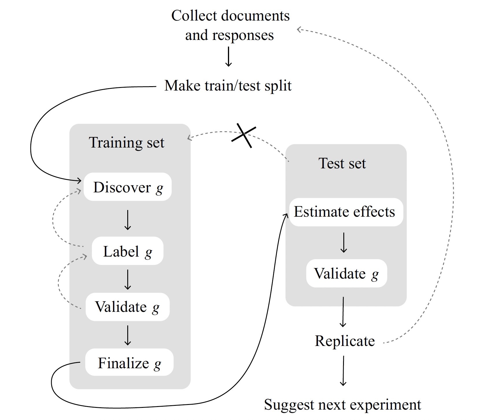
The Solution? Sample Splitting!

• Machine learning noticed this long ago: the goal is a model that generalizes, not memorizes!

References

Bamman, David, Brendan O’Connor, and Noah A. Smith. 2013. “Learning Latent Personas of Film Characters.” In Proceedings of the 51st Annual Meeting of the Association for Computational Linguistics (Volume 1: Long Papers), edited by Hinrich Schuetze, Pascale Fung, and Massimo Poesio. Association for Computational Linguistics. https://aclanthology.org/P13-1035/.

Egami, Naoki, Christian J. Fong, Justin Grimmer, Margaret E. Roberts, and Brandon M. Stewart. 2022. “How to Make Causal Inferences Using Texts.” Science Advances 8 (42): eabg2652. https://doi.org/10.1126/sciadv.abg2652.

Imai, Kosuke. 2018. Quantitative Social Science: An Introduction. Princeton University Press. https://books.google.com?id=T3GYDwAAQBAJ.

Nunn, Nathan, and Diego Puga. 2012. “Ruggedness: The Blessing of Bad Geography in Africa.” The Review of Economics and Statistics 94 (1): 20–36. https://www.jstor.org/stable/41349158.