Week 3: Getting Fancy with Regression
DSAN 5300: Statistical Learning
Spring 2026, Georgetown University
Monday, January 26, 2026
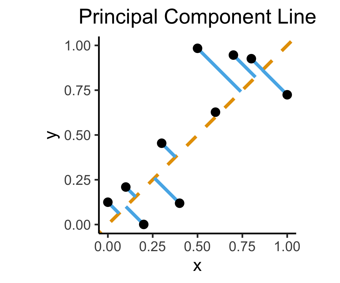
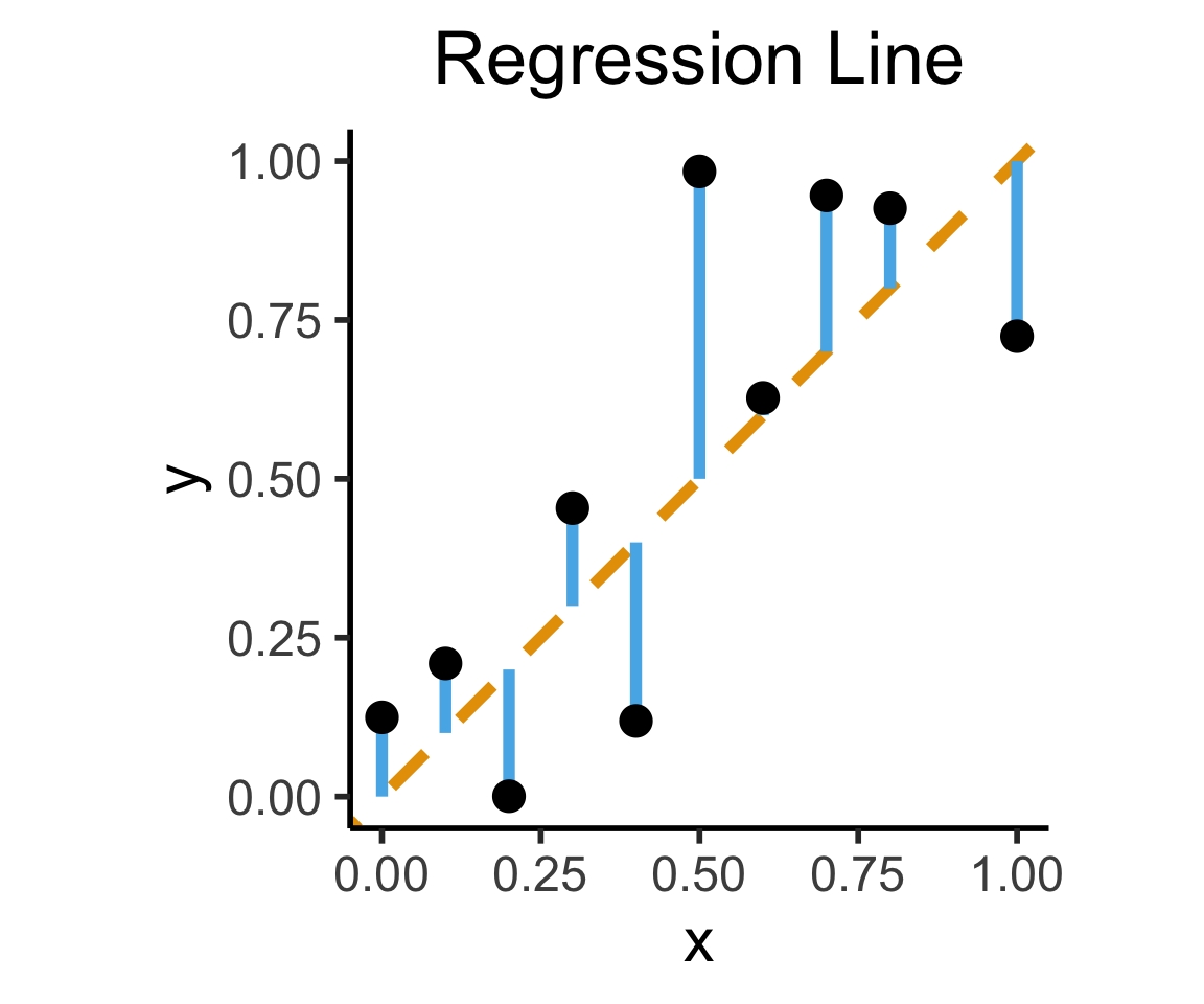
How Do We Define “Best”?
- Intuitively, two different ways to measure how well a line fits the data:
Code
library(tidyverse)
set.seed(5321)
N <- 11
x <- seq(from = 0, to = 1, by = 1 / (N - 1))
y <- x + rnorm(N, 0, 0.2)
mean_y <- mean(y)
spread <- y - mean_y
df <- tibble(x = x, y = y, spread = spread)
ggplot(df, aes(x=x, y=y)) +
  geom_abline(slope=1, intercept=0, linetype="dashed", color=cbPalette[1], linewidth=g_linewidth*2) +
  geom_segment(xend=(x+y)/2, yend=(x+y)/2, linewidth=g_linewidth*2, color=cbPalette[2]) +
  geom_point(size=g_pointsize) +
  coord_equal() +
  xlim(0, 1) + ylim(0, 1) +
  dsan_theme("half") +
  labs(
    title = "Principal Component Line"
  )
ggplot(df, aes(x=x, y=y)) +
  geom_abline(slope=1, intercept=0, linetype="dashed", color=cbPalette[1], linewidth=g_linewidth*2) +
  geom_segment(xend=x, yend=x, linewidth=g_linewidth*2, color=cbPalette[2]) +
  geom_point(size=g_pointsize) +
  coord_equal() +
  xlim(0, 1) + ylim(0, 1) +
  dsan_theme("half") +
  labs(
    title = "Regression Line"
  )
A Sketch
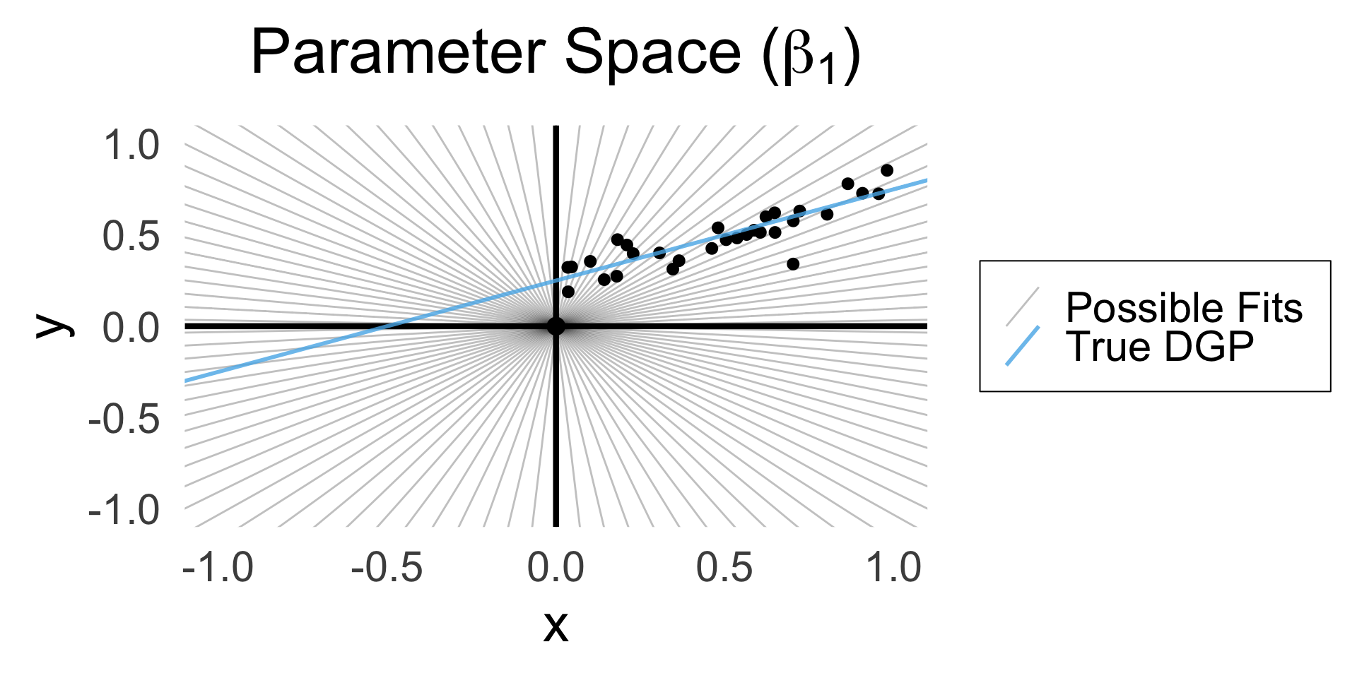
- OLS for regression without intercept: Which line through origin best predicts \(Y\)?
- (Good practice + reminder of how restricted linear models are!)
\[ Y = \beta_1 X + \varepsilon \]
Code
library(latex2exp)
set.seed(5300)
# rand_slope <- log(runif(80, min=0, max=1))
# rand_slope[41:80] <- -rand_slope[41:80]
# rand_lines <- tibble::tibble(
#   id=1:80, slope=rand_slope, intercept=0
# )
# angles <- runif(100, -pi/2, pi/2)
angles <- seq(from=-pi/2, to=pi/2, length.out=50)
possible_lines <- tibble::tibble(
  slope=tan(angles), intercept=0
)
num_points <- 30
x_vals <- runif(num_points, 0, 1)
y0_vals <- 0.5 * x_vals + 0.25
y_noise <- rnorm(num_points, 0, 0.07)
y_vals <- y0_vals + y_noise
rand_df <- tibble::tibble(x=x_vals, y=y_vals)
title_exp <- TeX("Parameter Space ($\\beta_1$)")
# Main plot object
gen_lines_plot <- function(point_size=2.5) {
  lines_plot <- rand_df |> ggplot(aes(x=x, y=y)) +
    geom_point(size=point_size) +
    geom_hline(yintercept=0, linewidth=1.5) +
    geom_vline(xintercept=0, linewidth=1.5) +
    # Point at origin
    geom_point(data=data.frame(x=0, y=0), aes(x=x, y=y), size=4) +
    xlim(-1,1) +
    ylim(-1,1) +
    # coord_fixed() +
    theme_dsan_min(base_size=28)
  return(lines_plot)
}
main_lines_plot <- gen_lines_plot()
main_lines_plot +
  # Parameter space of possible lines
  geom_abline(
    data=possible_lines,
    aes(slope=slope, intercept=intercept, color='possible'),
    # linetype="dotted",
    # linewidth=0.75,
    alpha=0.25
  ) +
  # True DGP
  geom_abline(
    aes(
      slope=0.5,
      intercept=0.25,
      color='true'
    ), linewidth=1, alpha=0.8
  ) +
  scale_color_manual(
    element_blank(),
    values=c('possible'="black", 'true'=cb_palette[2]),
    labels=c('possible'="Possible Fits", 'true'="True DGP")
  ) +
  remove_legend_title() +
  labs(
    title=title_exp
  )
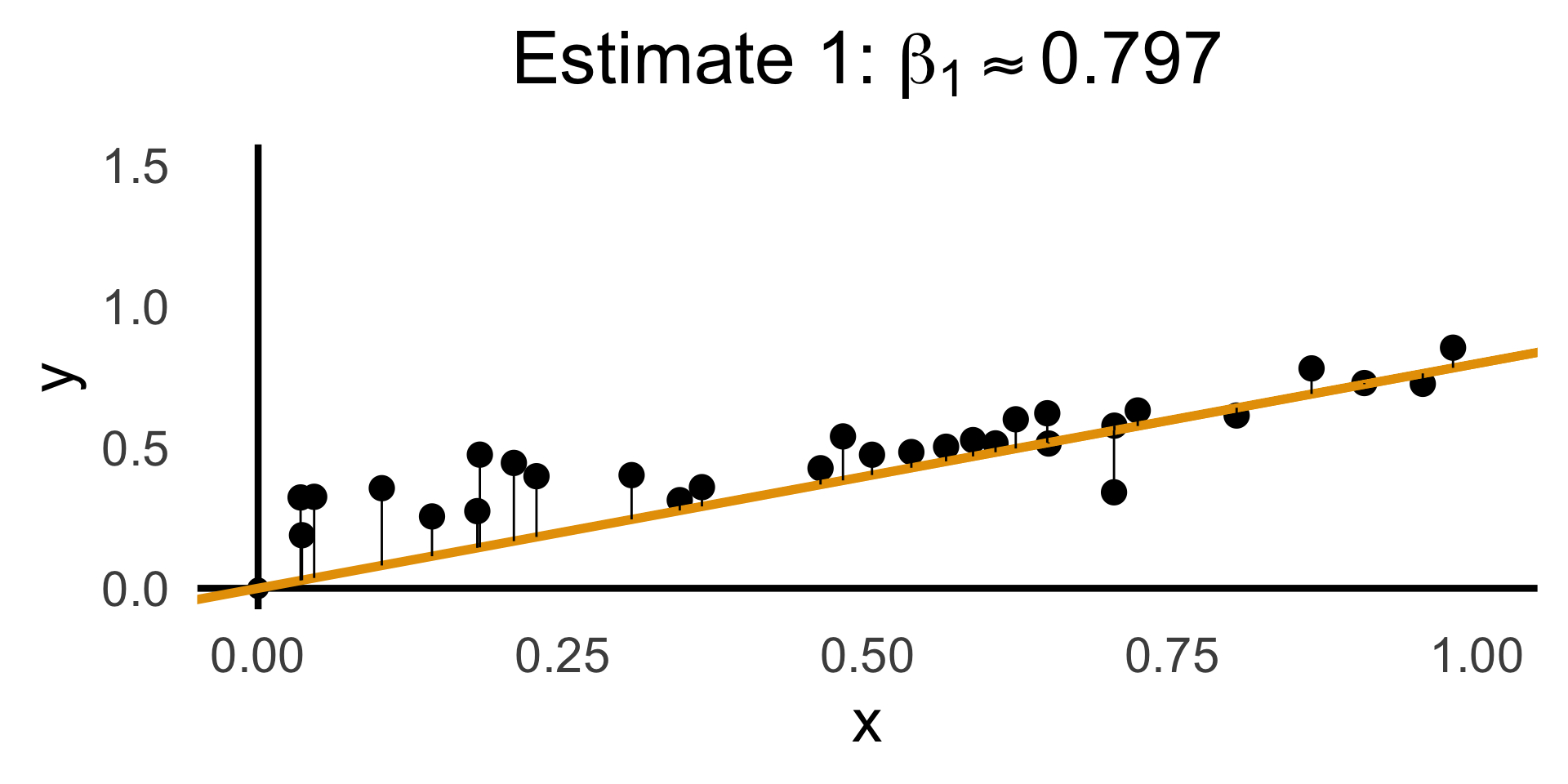
Evaluating with Residuals
Code
rc1_df <- possible_lines |> slice(n() - 14)
# Predictions for this choice
rc1_pred_df <- rand_df |> mutate(
  y_pred = rc1_df$slope * x,
  resid = y - y_pred
)
rc1_label <- TeX(paste0("Estimate 1: $\\beta_1 \\approx ",round(rc1_df$slope, 3),"$"))
rc1_lines_plot <- gen_lines_plot(point_size=5)
rc1_lines_plot +
  geom_abline(
    data=rc1_df,
    aes(intercept=intercept, slope=slope),
    linewidth=2,
    color=cb_palette[1]
  ) +
  geom_segment(
    data=rc1_pred_df,
    aes(x=x, y=y, xend=x, yend=y_pred),
    # color=cb_palette[1]
  ) +
  xlim(0, 1) + ylim(0, 1.5) +
  labs(
    title = rc1_label
  )
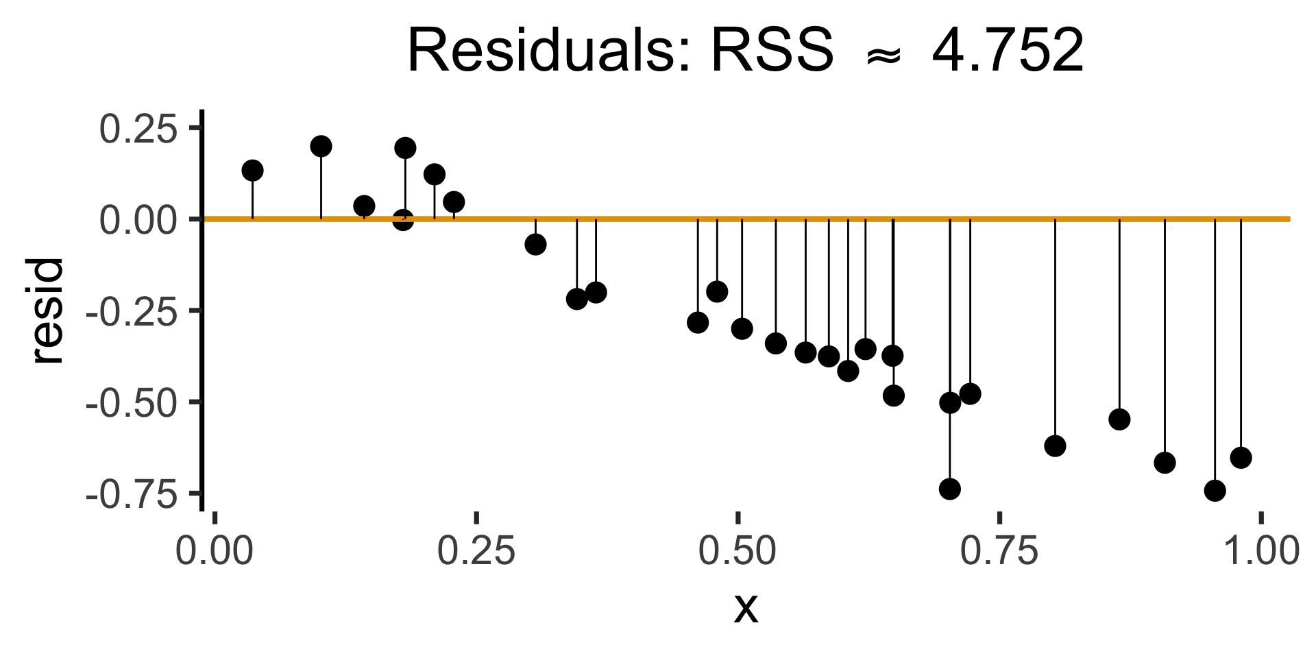
Code
gen_resid_plot <- function(pred_df) {
  rc_rss <- sum((pred_df$resid)^2)
  rc_resid_label <- TeX(paste0("Residuals: RSS $\\approx$ ",round(rc_rss,3)))
  rc_resid_plot <- pred_df |> ggplot(aes(x=x, y=resid)) +
    geom_point(size=5) +
    geom_hline(
      yintercept=0,
      color=cb_palette[1],
      linewidth=1.5
    ) +
    geom_segment(
      aes(xend=x, yend=0)
    ) +
    theme_dsan(base_size=28) +
    theme(axis.line.x = element_blank()) +
    ylim(-0.75, 0.25) +
    labs(
      title=rc_resid_label
    )
  return(rc_resid_plot)
}
rc1_resid_plot <- gen_resid_plot(rc1_pred_df)
rc1_resid_plot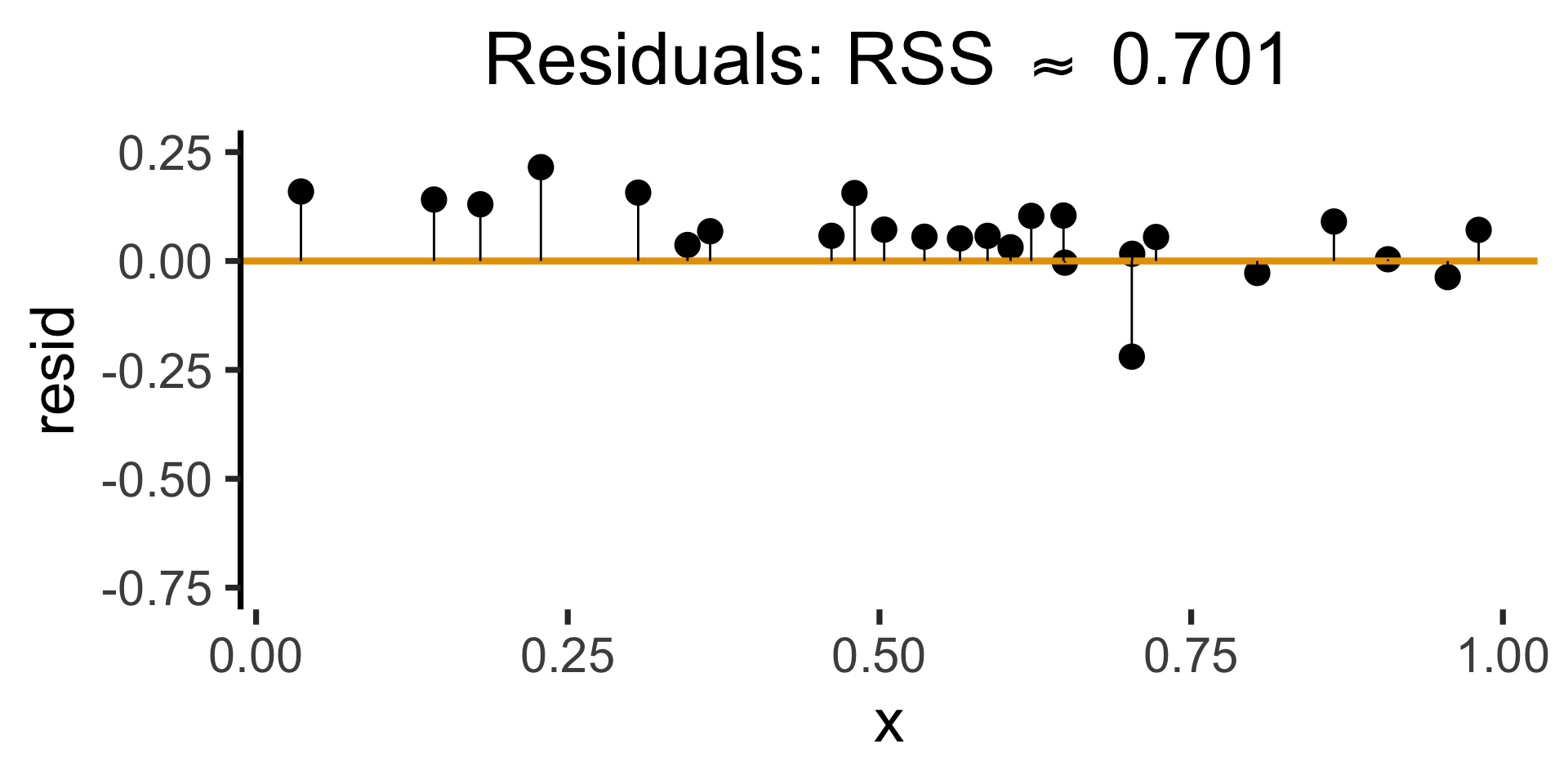
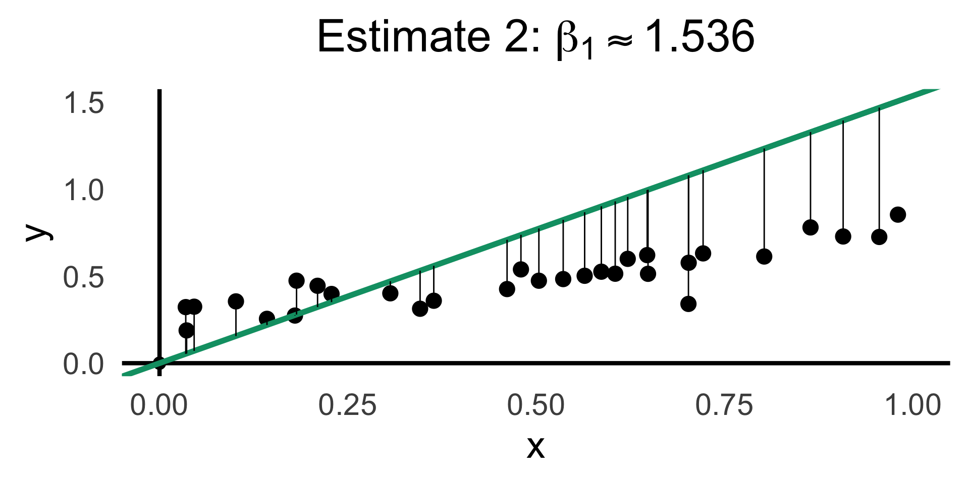
Code
rc2_df <- possible_lines |> slice(n() - 9)
# Predictions for this choice
rc2_pred_df <- rand_df |> mutate(
  y_pred = rc2_df$slope * x,
  resid = y - y_pred
)
rc2_label <- TeX(paste0("Estimate 2: $\\beta_1 \\approx ",round(rc2_df$slope,3),"$"))
rc2_lines_plot <- gen_lines_plot(point_size=5)
rc2_lines_plot +
  geom_abline(
    data=rc2_df,
    aes(intercept=intercept, slope=slope),
    linewidth=2,
    color=cb_palette[3]
  ) +
  geom_segment(
    data=rc2_pred_df,
    aes(
      x=x, y=y, xend=x,
      # yend=ifelse(y_pred <= 1, y_pred, Inf)
      yend=y_pred
    )
    # color=cb_palette[1]
  ) +
  xlim(0, 1) + ylim(0, 1.5) +
  labs(
    title=rc2_label
  )
Interpreting Output
Code
library(tidyverse)
gdp_df <- read_csv("assets/gdp_pca.csv")
mil_plot <- gdp_df |> ggplot(aes(x=industrial, y=military)) +
  geom_point(size=0.5*g_pointsize) +
  geom_smooth(method='lm', formula="y ~ x", linewidth=1) +
  theme_dsan() +
  labs(
    title="Military Exports vs. Industrialization",
    x="Industrial Production (% of GDP)",
    y="Military Exports (% of All Exports)"
  )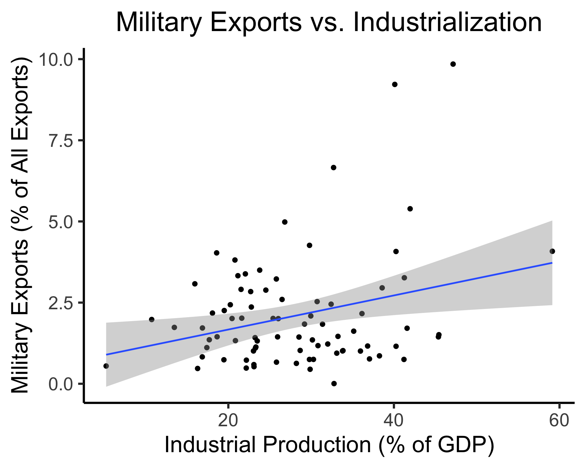
Call:
lm(formula = military ~ industrial, data = gdp_df)

Residuals:
    Min      1Q  Median      3Q     Max
-2.3354 -1.0997 -0.3870  0.6081  6.7508

Coefficients:
            Estimate Std. Error t value Pr(>|t|)
(Intercept)  0.61969    0.59526   1.041   0.3010
industrial   0.05253    0.02019   2.602   0.0111 *
---
Signif. codes:  0 '***' 0.001 '**' 0.01 '*' 0.05 '.' 0.1 ' ' 1

Residual standard error: 1.671 on 79 degrees of freedom
  (8 observations deleted due to missingness)
Multiple R-squared:  0.07895,   Adjusted R-squared:  0.06729
F-statistic: 6.771 on 1 and 79 DF,  p-value: 0.01106
Zooming In: Significance
| Estimate | Std. Error | t value | Pr(>|t|) | ||
|---|---|---|---|---|---|
| (Intercept) | 0.61969 | 0.59526 | 1.041 | 0.3010 | |
| industrial | 0.05253 | 0.02019 | 2.602 | 0.0111 | * |
| \(\widehat{\beta}\) | Uncertainty | Test stat \(t\) | How extreme is \(t\)? | Signif. Level |
Code
library(ggplot2)
int_tstat <- 1.041
int_tstat_str <- sprintf("%.02f", int_tstat)
label_df_int <- tribble(
    ~x, ~y, ~label,
    0.25, 0.05, paste0("P(t > ",int_tstat_str,")\n= 0.3")
)
label_df_signif_int <- tribble(
    ~x, ~y, ~label,
    2.7, 0.075, "95% Signif.\nCutoff"
)
funcShaded <- function(x, lower_bound, upper_bound){
    y <- dnorm(x)
    y[x < lower_bound | x > upper_bound] <- NA
    return(y)
}
funcShadedIntercept <- function(x) funcShaded(x, int_tstat, Inf)
funcShadedSignif <- function(x) funcShaded(x, 1.96, Inf)
ggplot(data=data.frame(x=c(-3,3)), aes(x=x)) +
  stat_function(fun=dnorm, linewidth=g_linewidth) +
  geom_vline(aes(xintercept=int_tstat), linewidth=g_linewidth, linetype="dashed") +
  geom_vline(aes(xintercept = 1.96), linewidth=g_linewidth, linetype="solid") +
  stat_function(fun = funcShadedIntercept, geom = "area", fill = cbPalette[1], alpha = 0.5) +
  stat_function(fun = funcShadedSignif, geom = "area", fill = "grey", alpha = 0.333) +
  geom_text(label_df_int, mapping = aes(x = x, y = y, label = label), size = 10) +
  geom_text(label_df_signif_int, mapping = aes(x = x, y = y, label = label), size = 8) +
  # Add single additional tick
  scale_x_continuous(breaks=c(-2, 0, int_tstat, 2), labels=c("-2","0",int_tstat_str,"2")) +
  dsan_theme("quarter") +
  labs(
    title = "t Value for Intercept",
    x = "t",
    y = "Density"
  ) +
  theme(axis.text.x = element_text(colour = c("black", "black", cbPalette[1], "black")))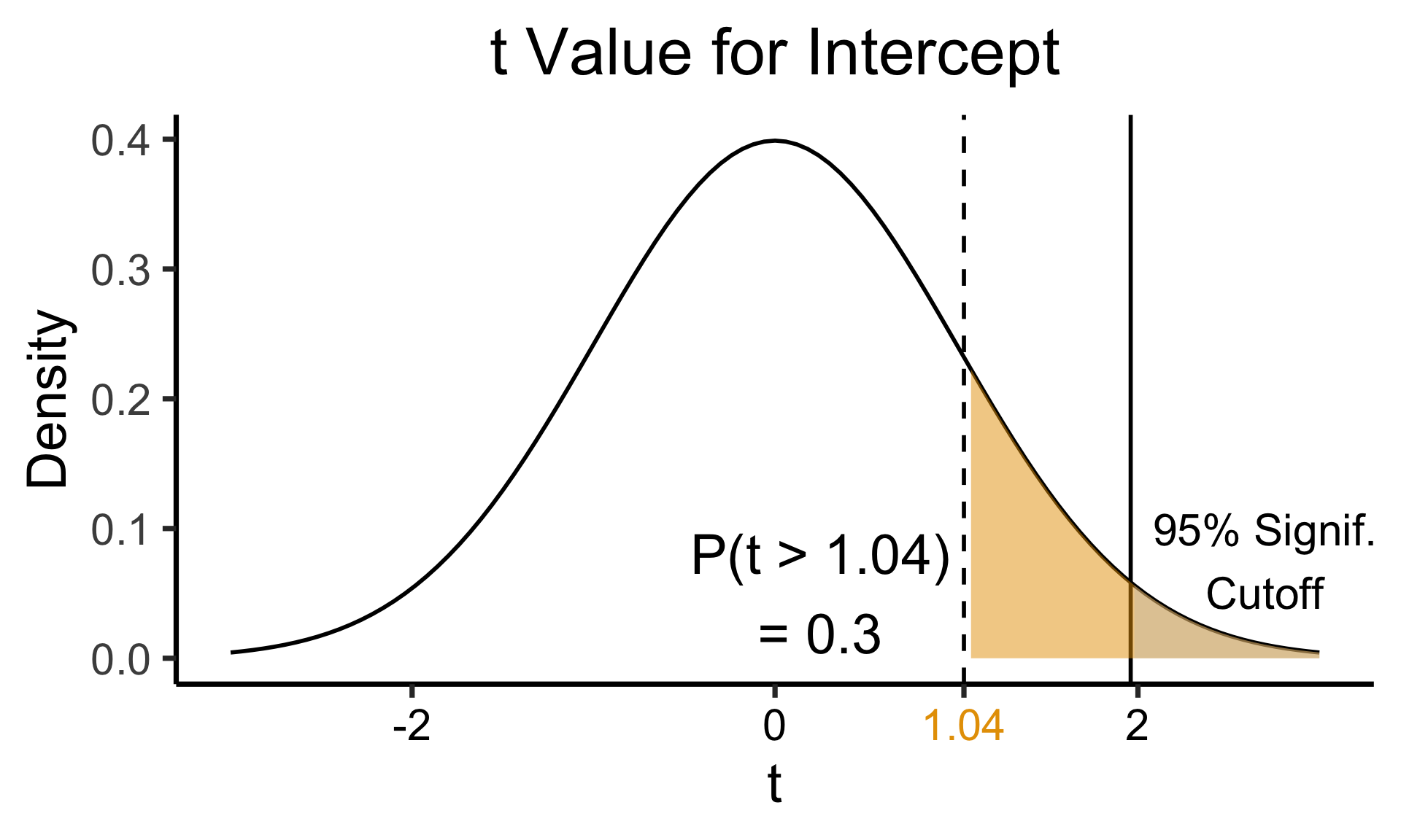
Code
library(ggplot2)
coef_tstat <- 2.602
coef_tstat_str <- sprintf("%.02f", coef_tstat)
label_df_coef <- tribble(
    ~x, ~y, ~label,
    3.65, 0.06, paste0("P(t > ",coef_tstat_str,")\n= 0.01")
)
label_df_signif_coef <- tribble(
  ~x, ~y, ~label,
  1.05, 0.03, "95% Signif.\nCutoff"
)
funcShadedCoef <- function(x) funcShaded(x, coef_tstat, Inf)
ggplot(data=data.frame(x=c(-4,4)), aes(x=x)) +
  stat_function(fun=dnorm, linewidth=g_linewidth) +
  geom_vline(aes(xintercept=coef_tstat), linetype="dashed", linewidth=g_linewidth) +
  geom_vline(aes(xintercept=1.96), linetype="solid", linewidth=g_linewidth) +
  stat_function(fun = funcShadedCoef, geom = "area", fill = cbPalette[2], alpha = 0.5) +
  stat_function(fun = funcShadedSignif, geom = "area", fill = "grey", alpha = 0.333) +
  # Label shaded area
  geom_text(label_df_coef, mapping = aes(x = x, y = y, label = label), size = 10) +
  # Label significance cutoff
  geom_text(label_df_signif_coef, mapping = aes(x = x, y = y, label = label), size = 8) +
  coord_cartesian(clip = "off") +
  # Add single additional tick
  scale_x_continuous(breaks=c(-4, -2, 0, 2, coef_tstat, 4), labels=c("-4", "-2","0", "2", coef_tstat_str,"4")) +
  dsan_theme("quarter") +
  labs(
    title = "t Value for Coefficient",
    x = "t",
    y = "Density"
  ) +
  theme(axis.text.x = element_text(colour = c("black", "black", "black", "black", cbPalette[2], "black")))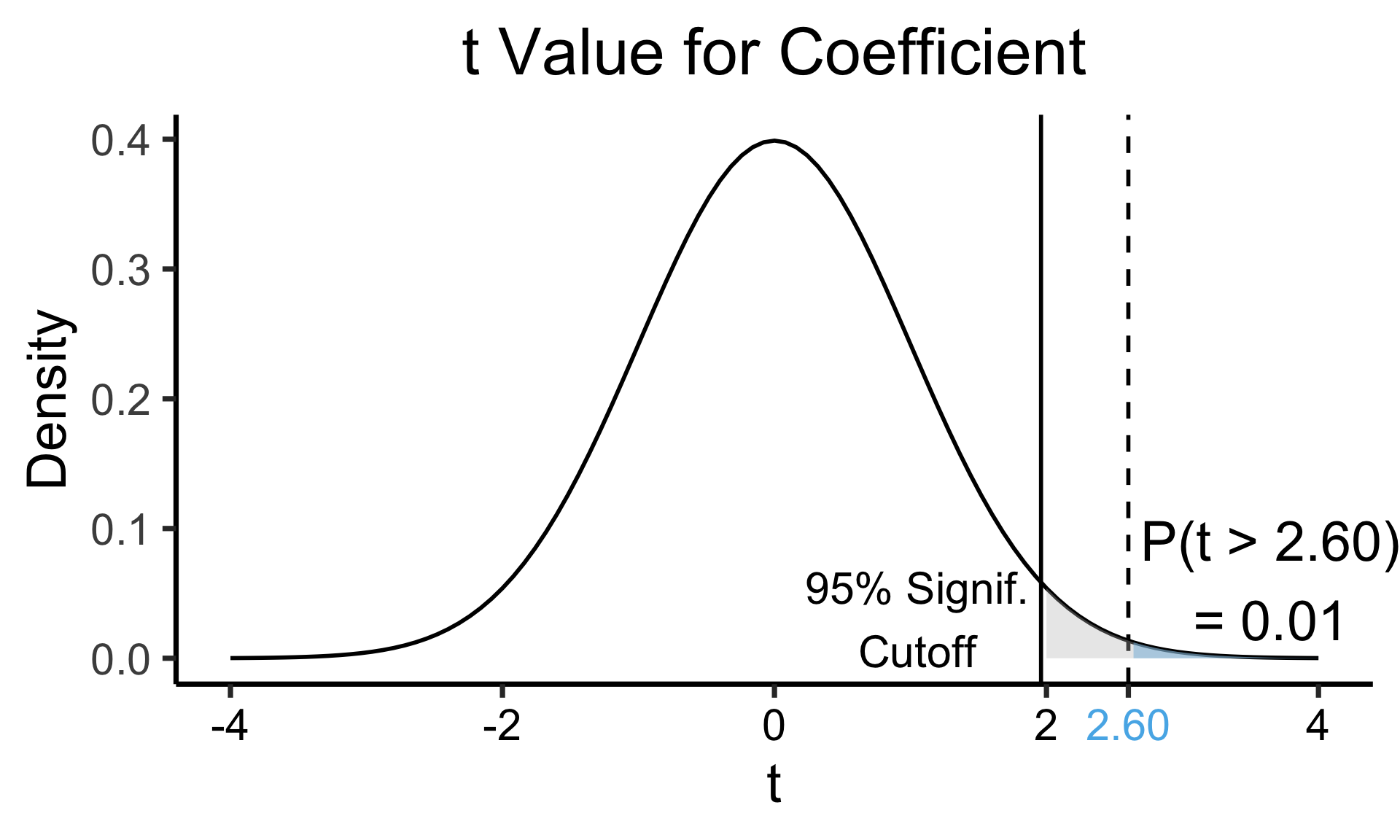
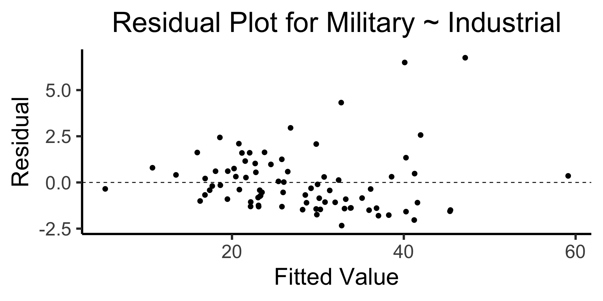
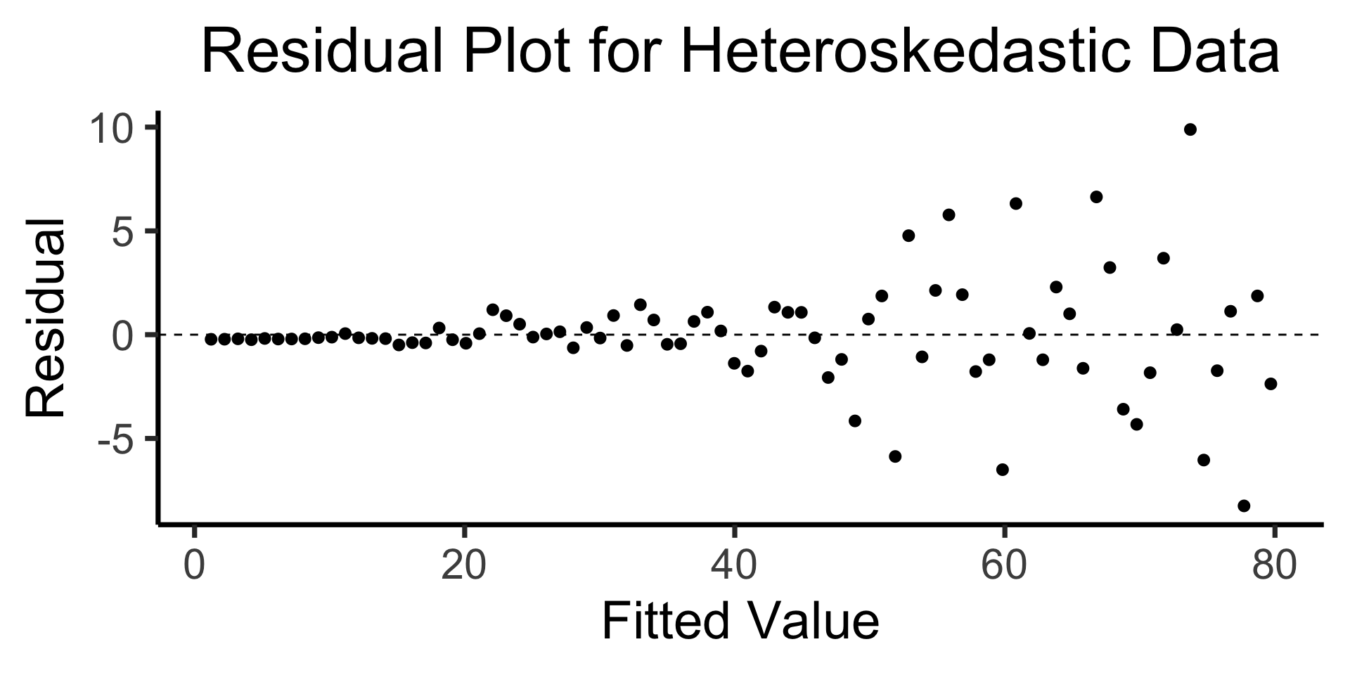
The Residual Plot
Recall homoskedasticity assumption: Given our model
\[ y_i = \beta_0 + \beta_1x_i + \varepsilon_i \]
the errors \(\varepsilon_i\) should not vary systematically with \(i\)
Formally: \(\forall i \left[ \Var{\varepsilon_i} = \sigma^2 \right]\)
Code
library(broom)
gdp_resid_df <- augment(gdp_model)
ggplot(gdp_resid_df, aes(x = industrial, y = .resid)) +
    geom_point(size = g_pointsize/2) +
    geom_hline(yintercept=0, linetype="dashed") +
    dsan_theme("quarter") +
    labs(
      title = "Residual Plot for Military ~ Industrial",
      x = "Fitted Value",
      y = "Residual"
    )
Code
x <- 1:80
errors <- rnorm(length(x), 0, x^2/1000)
y <- x + errors
het_model <- lm(y ~ x)
df_het <- augment(het_model)
ggplot(df_het, aes(x = .fitted, y = .resid)) +
    geom_point(size = g_pointsize / 2) +
    geom_hline(yintercept = 0, linetype = "dashed") +
    dsan_theme("quarter") +
    labs(
        title = "Residual Plot for Heteroskedastic Data",
        x = "Fitted Value",
        y = "Residual"
    )
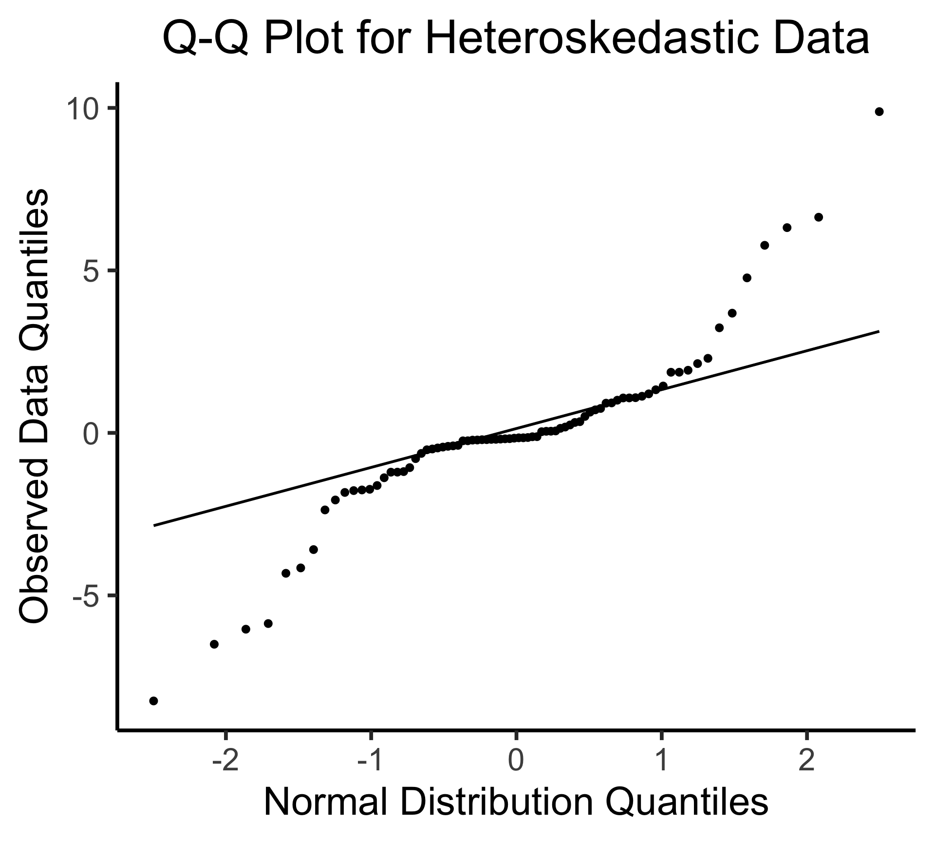
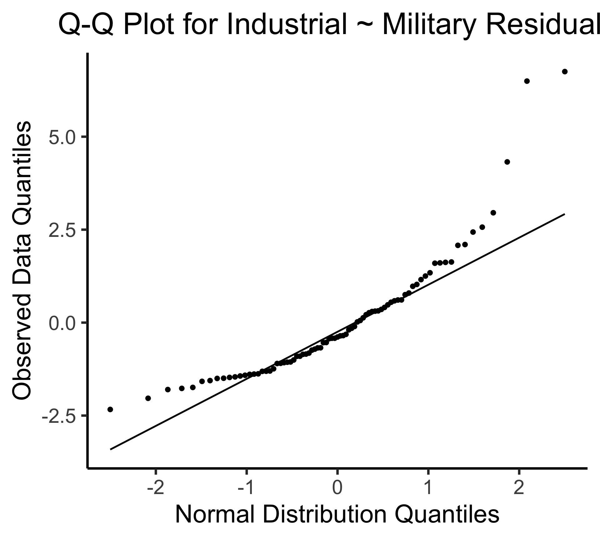
Q-Q Plot
- If \((\widehat{y} - y) \sim \mathcal{N}(0, \sigma^2)\), points would lie on 45° line:
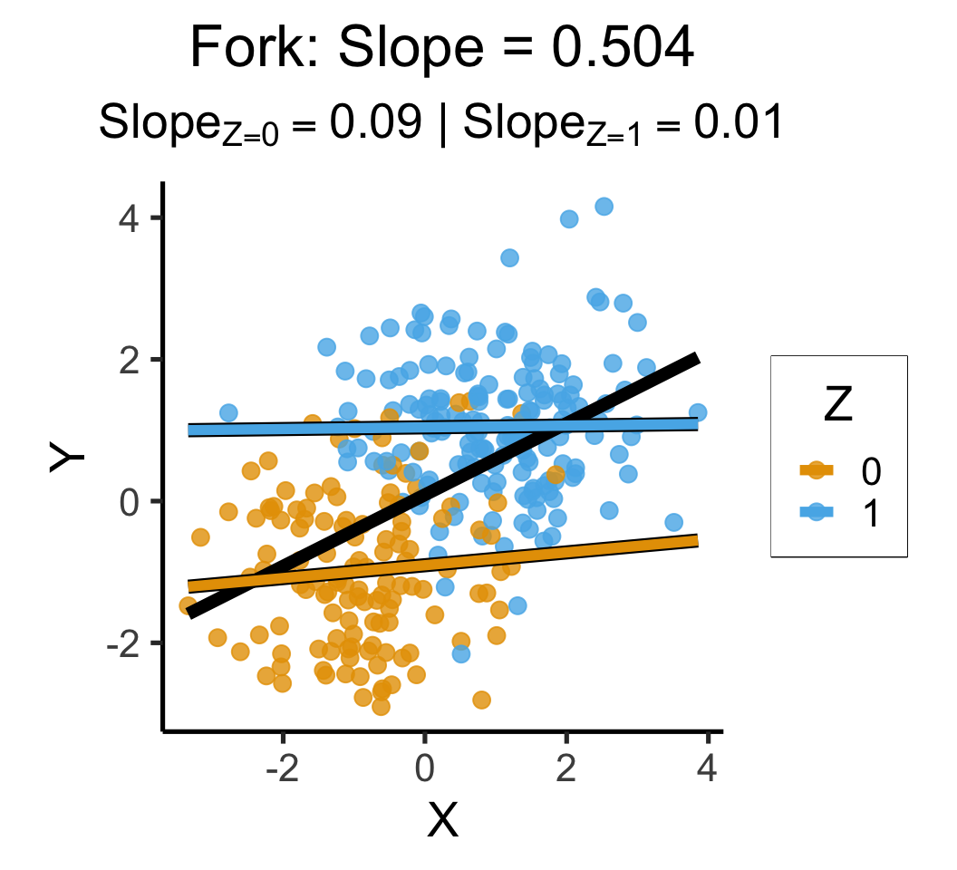
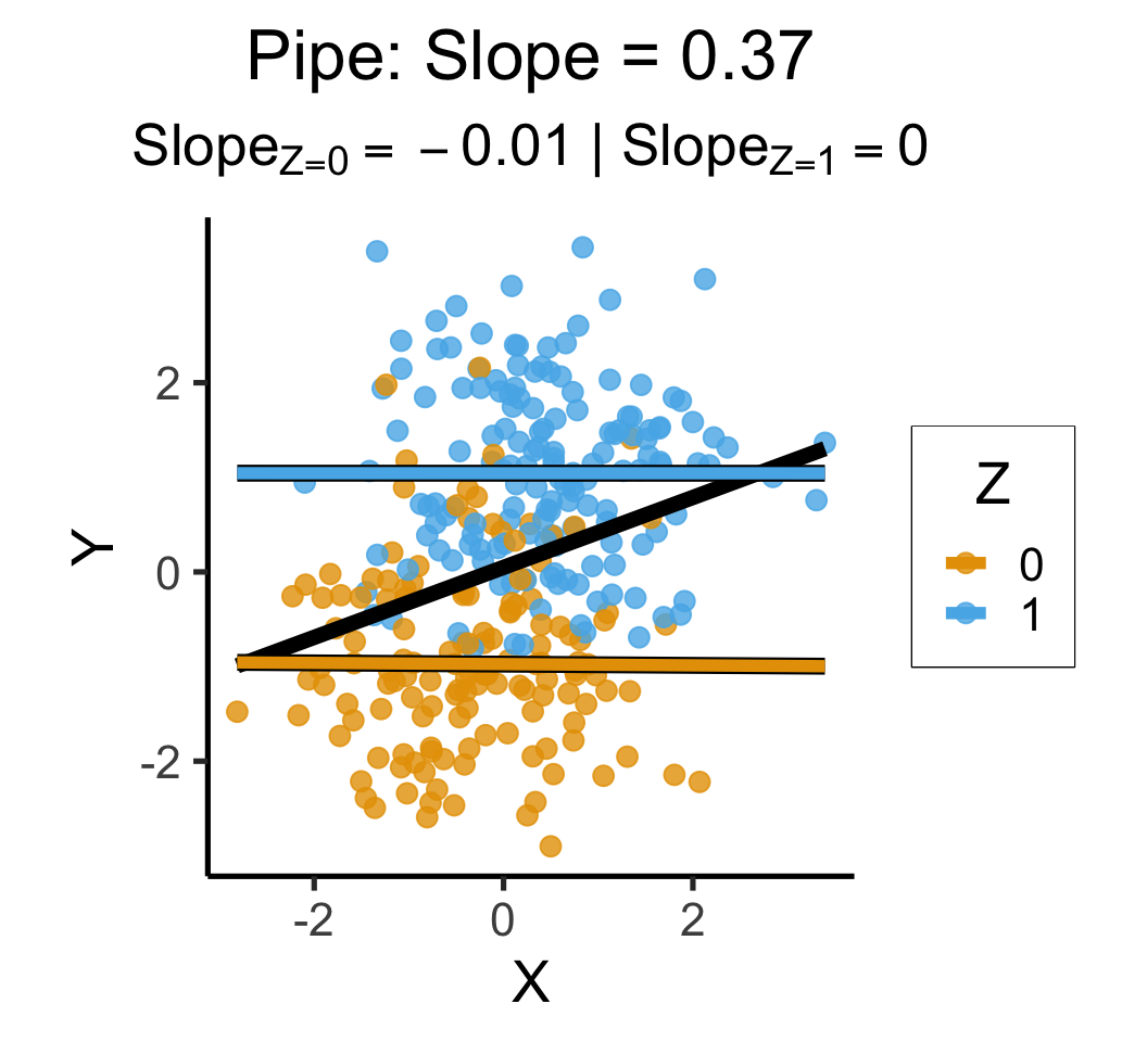
“Holding” Things “Constant”?
- One of the more confusing ideas in all of statistics…
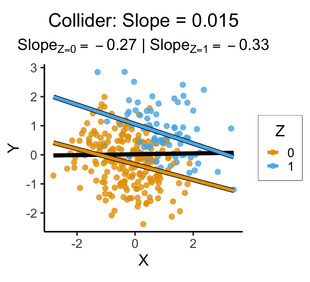
- “Controlling for” some types of variables (forks, pipes) removes spurious correlation, but “controlling for” other types (colliders) introduces more spurious correlation
- Opinionated “what you should really do”: center independent variables
- \(Y = \beta_0 + \beta_1 (X - \mu)\) \(\Rightarrow\) “When other variables are at their mean values, 1 unit increase in \(X_i\) associated with \(\beta_i\) unit increase in \(y\)”
Code
library(extraDistr)
set.seed(5650)
n_c <- 300
cfork_df <- tibble(
    Z = rbern(n_c),
    X = rnorm(n_c, 2 * Z - 1),
    Y = rnorm(n_c, 2 * Z - 1)
)
library(latex2exp)
overall_lm <- lm(Y ~ X, data=cfork_df)
overall_slope <- round(overall_lm$coef['X'], 3)
z0_lm <- lm(Y ~ X, data=cfork_df |> filter(Z == 0))
z0_slope <- round(z0_lm$coef['X'], 2)
z0_label <- paste0("$Slope_{Z=0} = ",z0_slope,"$")
z0_leg_label <- TeX(paste0("0 $(m=",z0_slope,")$"))
z1_lm <- lm(Y ~ X, data=cfork_df |> filter(Z == 1))
z1_slope <- round(z1_lm$coef['X'], 2)
z1_label <- paste0("$Slope_{Z=1} = ",z1_slope,"$")
z_texlabel <- TeX(paste0(z0_label, " | ", z1_label))
cfork_xmin <- min(cfork_df$X)
cfork_xmax <- max(cfork_df$X)
ggplot() +
  # Points
  geom_point(
    data=cfork_df,
    aes(x=X, y=Y, color=factor(Z)),
    size=0.6*g_pointsize,
    alpha=0.8
  ) +
  # Overall lm
  geom_smooth(
    data=cfork_df, aes(x=X, y=Y),
    method = lm, se = FALSE,
    linewidth = 2.5, color='black'
  ) +
  # Stratified lm
  # (slightly larger black lines)
  geom_smooth(
    data=cfork_df,
    aes(x=X, y=Y, group=factor(Z)),
    method=lm, se=FALSE, fullrange=TRUE,
    linewidth=2.75, color='black'
  ) +
  # (Colored lines)
  geom_smooth(
    data=cfork_df,
    aes(x=X, y=Y, color=factor(Z)),
    method=lm, se=FALSE, fullrange=TRUE,
    linewidth=2
  ) +
  theme_dsan(base_size=20) +
  theme(
    plot.title = element_text(size=24),
    plot.subtitle = element_text(size=20)
  ) +
  coord_equal() +
  labs(
    title = paste0(
      "Fork: Slope = ",overall_slope
    ),
    subtitle=z_texlabel,
    x = "X", y = "Y", color = "Z"
  )
set.seed(5650)
cpipe_df <- tibble(
    X = rnorm(n_c),
    Z = rbern(n_c, plogis(X)),
    Y = rnorm(n_c, 2 * Z - 1)
)
cpipe_lm <- lm(Y ~ X, data=cpipe_df)
cpipe_slope <- round(cpipe_lm$coef['X'], 3)
cpipe_z0_lm <- lm(Y ~ X, data=cpipe_df |> filter(Z == 0))
cpipe_z0_slope <- round(cpipe_z0_lm$coef['X'], 2)
cpipe_z0_label <- paste0("$Slope_{Z=0} = ",cpipe_z0_slope,"$")
cpipe_z1_lm <- lm(Y ~ X, data=cpipe_df |> filter(Z == 1))
cpipe_z1_slope <- round(cpipe_z1_lm$coef['X'], 2)
cpipe_z1_label <- paste0("$Slope_{Z=1} = ",cpipe_z1_slope,"$")
cpipe_z_texlabel <- TeX(paste0(cpipe_z0_label, " | ", cpipe_z1_label))
cpipe_xmin <- min(cpipe_df$X)
cpipe_xmax <- max(cpipe_df$X)
ggplot() +
  # Points
  geom_point(
    data=cpipe_df |> filter(Y > -3),
    aes(x=X, y=Y, color=factor(Z)),
    size=0.6*g_pointsize,
    alpha=0.8
  ) +
  # Overall lm
  geom_smooth(
    data=cpipe_df, aes(x=X, y=Y),
    method = lm, se = FALSE,
    linewidth = 2.5, color='black'
  ) +
  # Stratified lm
  # (slightly larger black lines)
  geom_smooth(
    data=cpipe_df,
    aes(x=X, y=Y, group=factor(Z)),
    method=lm, se=FALSE, fullrange=TRUE,
    linewidth=2.75, color='black'
  ) +
  # (Colored lines)
  geom_smooth(
    data=cpipe_df,
    aes(x=X, y=Y, color=factor(Z)),
    method=lm, se=FALSE, fullrange=TRUE,
    linewidth=2
  ) +
  theme_dsan(base_size=20) +
  theme(
    plot.title = element_text(size=24),
    plot.subtitle = element_text(size=20)
  ) +
  coord_equal() +
  labs(
    title = paste0(
      "Pipe: Slope = ",cpipe_slope
    ),
    subtitle=cpipe_z_texlabel,
    x = "X", y = "Y", color = "Z"
  )
set.seed(5650)
ccoll_df <- tibble(
    X = rnorm(n_c),
    Y = rnorm(n_c),
    Z = rbern(n_c, plogis(2 * (X + Y - 1)))
)
ccoll_lm <- lm(Y ~ X, data=ccoll_df)
ccoll_slope <- round(ccoll_lm$coef['X'], 3)
ccoll_z0_lm <- lm(Y ~ X, data=ccoll_df |> filter(Z == 0))
ccoll_z0_slope <- round(ccoll_z0_lm$coef['X'], 2)
ccoll_z0_label <- paste0("$Slope_{Z=0} = ",ccoll_z0_slope,"$")
ccoll_z1_lm <- lm(Y ~ X, data=ccoll_df |> filter(Z == 1))
ccoll_z1_slope <- round(ccoll_z1_lm$coef['X'], 2)
ccoll_z1_label <- paste0("$Slope_{Z=1} = ",ccoll_z1_slope,"$")
ccoll_z_texlabel <- TeX(paste0(ccoll_z0_label, " | ", ccoll_z1_label))
ccoll_xmin <- min(ccoll_df$X)
ccoll_xmax <- max(ccoll_df$X)
ggplot() +
  # Points
  geom_point(
    data=ccoll_df |> filter(Y > -3),
    aes(x=X, y=Y, color=factor(Z)),
    size=0.6*g_pointsize,
    alpha=0.8
  ) +
  # Overall lm
  geom_smooth(
    data=ccoll_df, aes(x=X, y=Y),
    method = lm, se = FALSE,
    linewidth = 2.5, color='black'
  ) +
  # Stratified lm
  # (slightly larger black lines)
  geom_smooth(
    data=ccoll_df,
    aes(x=X, y=Y, group=factor(Z)),
    method=lm, se=FALSE, fullrange=TRUE,
    linewidth=2.75, color='black'
  ) +
  # (Colored lines)
  geom_smooth(
    data=ccoll_df,
    aes(x=X, y=Y, color=factor(Z)),
    method=lm, se=FALSE, fullrange=TRUE,
    linewidth=2
  ) +
  theme_dsan(base_size=20) +
  theme(
    plot.title = element_text(size=24),
    plot.subtitle = element_text(size=20)
  ) +
  coord_equal() +
  labs(
    title = paste0(
      "Collider: Slope = ",ccoll_slope
    ),
    subtitle=ccoll_z_texlabel,
    x = "X", y = "Y", color = "Z"
  )
Visualizing MLR

(ISLR, Fig 3.5): A pronounced non-linear relationship. Positive residuals (visible above the surface) tend to lie along the 45-degree line, where budgets are split evenly. Negative residuals (most not visible) tend to be away from this line, where budgets are more lopsided.
MLR Superpower: Handling Categorical Vars
\[ \begin{align*} Y &= \beta_0 + \beta_1 \times \texttt{income} \\ &\phantom{Y} \end{align*} \]
Code
credit_df <- read_csv("assets/Credit.csv")
credit_plot <- credit_df |> ggplot(aes(x=Income, y=Balance)) +
  geom_point(size=0.5*g_pointsize) +
  geom_smooth(
    method='lm', formula="y ~ x", linewidth=1,
    fullrange=TRUE
  ) +
  theme_dsan() +
  labs(
    title="Credit Card Balance vs. Income Level",
    x="Income ($1K)",
    y="Credit Card Balance ($)"
  )
credit_plot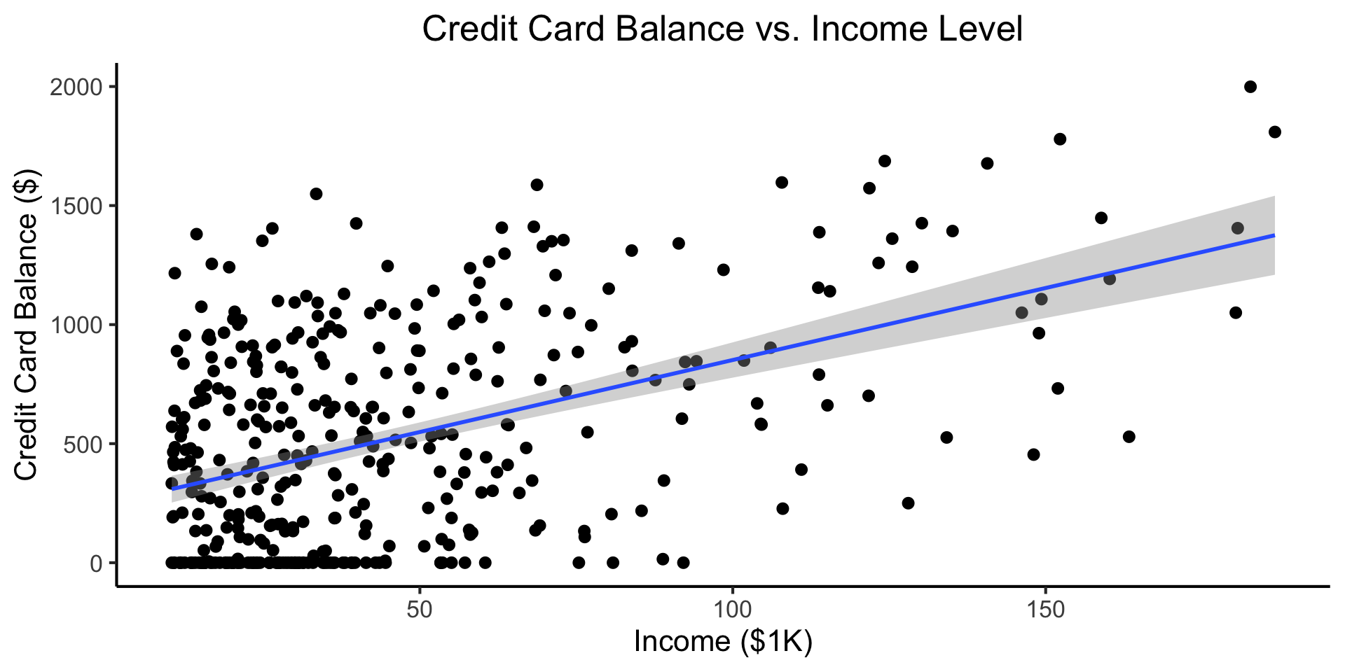
\[ \begin{align*} Y = &\beta_0 + \beta_1 \times \texttt{income} + \beta_2 \times \texttt{Student} \\ &+ \beta_3 \times (\texttt{Student} \times \texttt{Income}) \end{align*} \]
Code
student_plot <- credit_df |> ggplot(aes(x=Income, y=Balance, color=Student)) +
  geom_point(size=0.5*g_pointsize) +
  geom_smooth(
    method='lm', formula="y ~ x", linewidth=1,
    fullrange=TRUE
  ) +
  theme_dsan() +
  labs(
    title="Credit Card Balance vs. Income Level",
    x="Income ($1K)",
    y="Credit Card Balance ($)"
  )
student_plot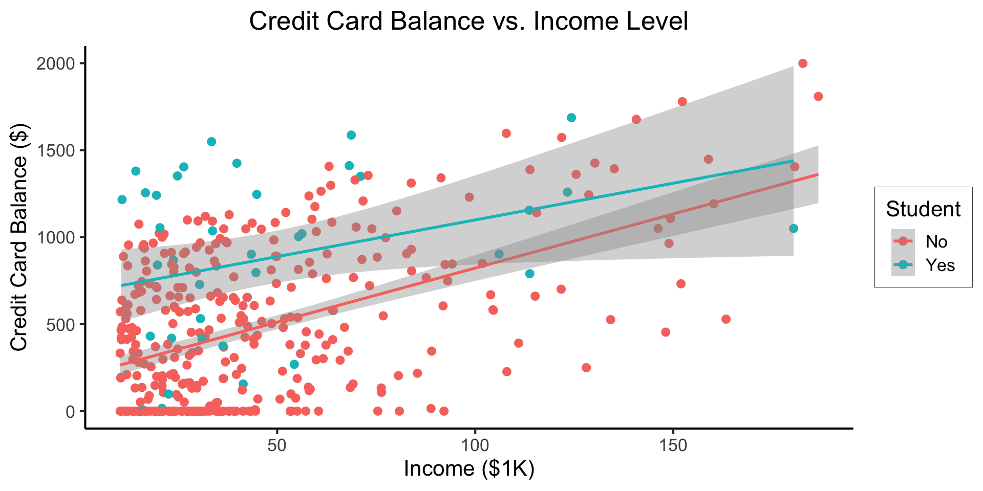
- Why do we need the \(\texttt{Student} \times \texttt{Income}\) term?
- Understanding this setup will open up a vast array of possibilities for regression 😎
- (Dear future Jeff, let’s go through this on the board! Sincerely, past Jeff)
From MLR to Logistic Regression
- As DSAN students, you know that we’re still sweeping classification under the rug!
- We saw how to include binary/multiclass covariates, but what if the actual thing we’re trying to predict is binary?
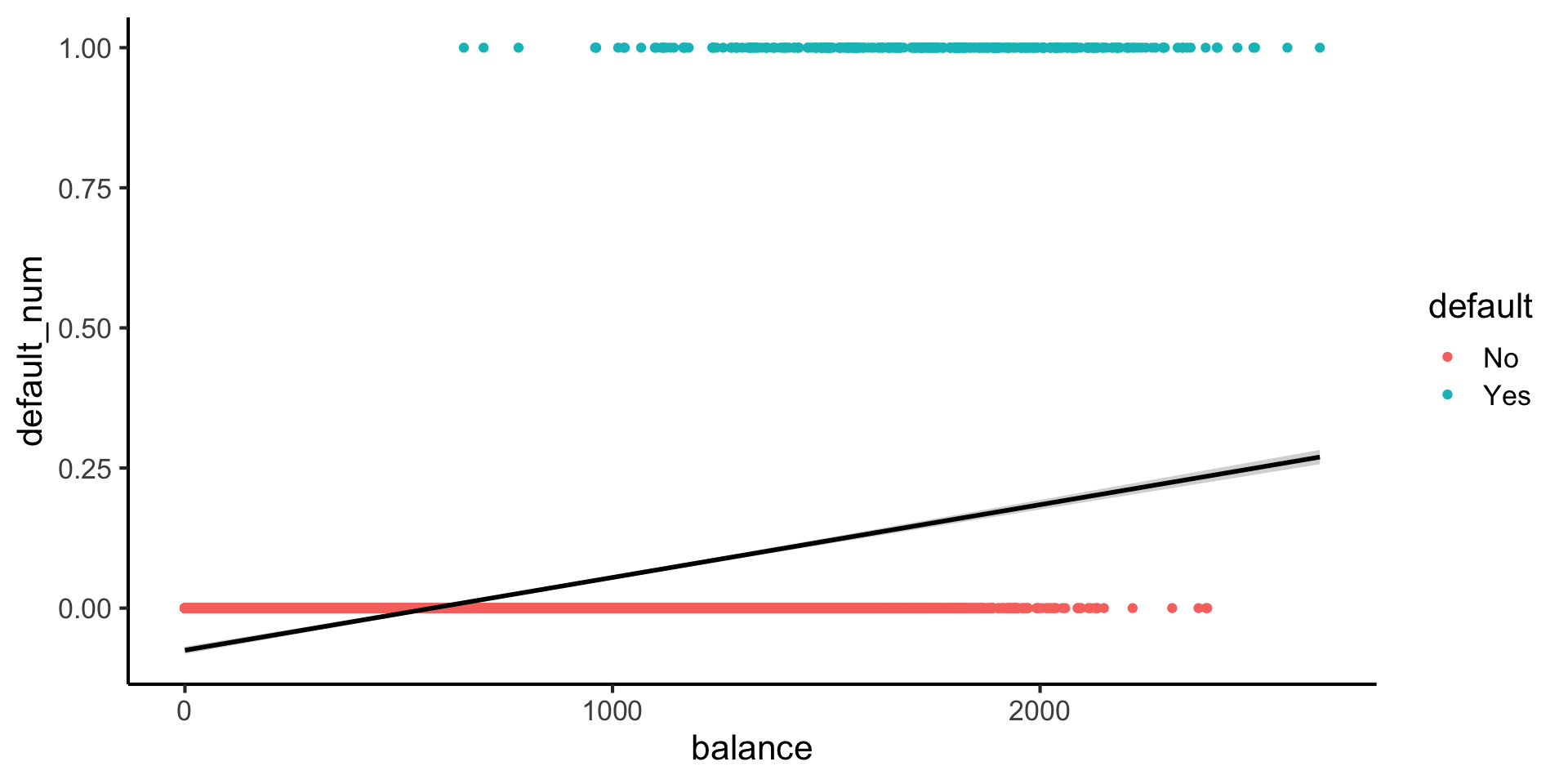
- The wrong approach is the “Linear Probability Model”:
\[ \Pr(Y \mid X) = \beta_0 + \beta_1 X + \varepsilon \]

Credit Default
Code
library(tidyverse)
library(ggExtra)
default_df <- read_csv("assets/Default.csv") |>
  mutate(default_num = ifelse(default=="Yes",1,0))
default_plot <- default_df |> ggplot(aes(x=balance, y=income, color=default, shape=default)) +
  geom_point(alpha=0.6) +
  theme_classic(base_size=16) +
  labs(
    title="Credit Defaults by Income and Account Balance",
    x = "Account Balance",
    y = "Income"
  )
default_mplot <- default_plot |> ggMarginal(type="boxplot", groupColour=FALSE, groupFill=TRUE)
default_mplot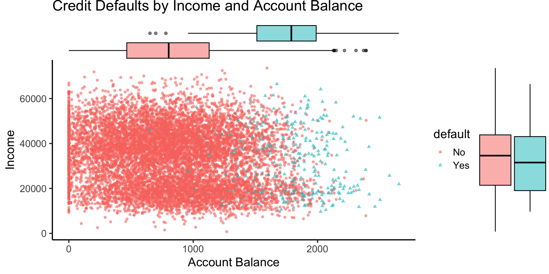
Lines vs. Sigmoids(!)
Here’s what lines look like for this dataset:
Here’s what sigmoids look like:
Code
library(tidyverse)
logistic_model <- glm(default_num ~ balance, family=binomial(link='logit'),data=default_df)
default_df$predictions <- predict(logistic_model, newdata = default_df, type = "response")
my_sigmoid <- function(x) 1 / (1+exp(-x))
default_df |> ggplot(aes(x=balance, y=default_num)) +
  #stat_function(fun=my_sigmoid) +
  geom_point(aes(color=default)) +
  geom_line(
    data=default_df,
    aes(x=balance, y=predictions),
    linewidth=1
  ) +
  theme_classic(base_size=16)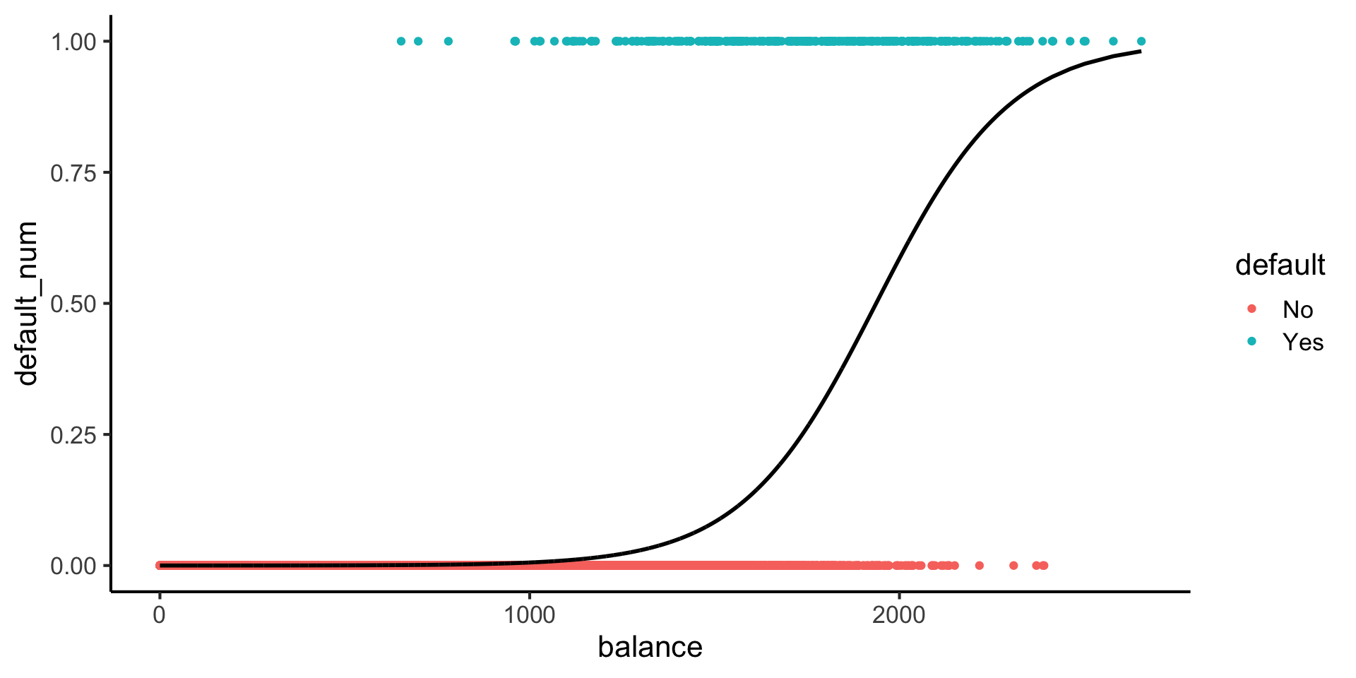
\[ \Pr(Y \mid X) = \beta_0 + \beta_1 X + \varepsilon \]
\[ \log\underbrace{\left[ \frac{\Pr(Y \mid X)}{1 - \Pr(Y \mid X)} \right]}_{\mathclap{\smash{\text{Odds Ratio}}}} = \beta_0 + \beta_1 X + \varepsilon \]