Week 2: Linear Regression

DSAN 5300: Statistical Learning
Spring 2026, Georgetown University

Jeff Jacobs

jj1088@georgetown.edu

Monday, January 12, 2026

Schedule

Today’s Planned Schedule:

	Start	End	Topic
Lecture	6:30pm	7:10pm	Simple Linear Regression →
	7:10pm	7:30pm	Deriving the OLS Solution →
	7:30pm	8:00pm	Interpreting OLS Output →
Break!	8:00pm	8:10pm
	8:10pm	8:30pm	Quiz Review →
	8:30pm	9:00pm	Quiz 2!

Linear Regression

• What happens to my dependent variable \(Y\) when my independent variable \(X\) increases by 1 unit?

• Keep the goal in front of your mind:

  The Goal of Regression

  Find a line \(\widehat{y} = mx + b\) that best predicts \(Y\) for given values of \(X\)

• Sanity Note 1: \(\Rightarrow\) measuring error via vertical distance from line
• Sanity Note 2: \(\Rightarrow\) modeling distribution of \(\boxed{Y \mid X}\), not \((X,Y)\)!
  • Predicting \(Y\) from \(X\) and \(X\) from \(Y\) \(\Rightarrow\) principal component line \(\neq\) regression!

\[ \DeclareMathOperator*{\argmax}{argmax} \DeclareMathOperator*{\argmin}{argmin} \newcommand{\bigexp}[1]{\exp\mkern-4mu\left[ #1 \right]} \newcommand{\bigexpect}[1]{\mathbb{E}\mkern-4mu \left[ #1 \right]} \newcommand{\definedas}{\overset{\small\text{def}}{=}} \newcommand{\definedalign}{\overset{\phantom{\text{defn}}}{=}} \newcommand{\eqeventual}{\overset{\text{eventually}}{=}} \newcommand{\Err}{\text{Err}} \newcommand{\expect}[1]{\mathbb{E}[#1]} \newcommand{\expectsq}[1]{\mathbb{E}^2[#1]} \newcommand{\fw}[1]{\texttt{#1}} \newcommand{\given}{\mid} \newcommand{\green}[1]{\color{green}{#1}} \newcommand{\heads}{\outcome{heads}} \newcommand{\iid}{\overset{\text{\small{iid}}}{\sim}} \newcommand{\lik}{\mathcal{L}} \newcommand{\loglik}{\ell} \DeclareMathOperator*{\maximize}{maximize} \DeclareMathOperator*{\minimize}{minimize} \newcommand{\mle}{\textsf{ML}} \newcommand{\nimplies}{\;\not\!\!\!\!\implies} \newcommand{\orange}[1]{\color{orange}{#1}} \newcommand{\outcome}[1]{\textsf{#1}} \newcommand{\param}[1]{{\color{purple} #1}} \newcommand{\pgsamplespace}{\{\green{1},\green{2},\green{3},\purp{4},\purp{5},\purp{6}\}} \newcommand{\pedge}[2]{\require{enclose}\enclose{circle}{~{#1}~} \rightarrow \; \enclose{circle}{\kern.01em {#2}~\kern.01em}} \newcommand{\pnode}[1]{\require{enclose}\enclose{circle}{\kern.1em {#1} \kern.1em}} \newcommand{\ponode}[1]{\require{enclose}\enclose{box}[background=lightgray]{{#1}}} \newcommand{\pnodesp}[1]{\require{enclose}\enclose{circle}{~{#1}~}} \newcommand{\purp}[1]{\color{purple}{#1}} \newcommand{\sign}{\text{Sign}} \newcommand{\spacecap}{\; \cap \;} \newcommand{\spacewedge}{\; \wedge \;} \newcommand{\tails}{\outcome{tails}} \newcommand{\Var}[1]{\text{Var}[#1]} \newcommand{\bigVar}[1]{\text{Var}\mkern-4mu \left[ #1 \right]} \]

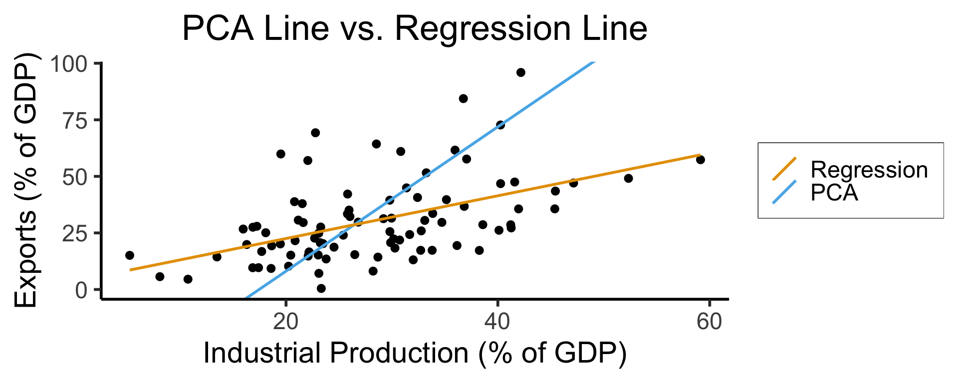
How Do We Define “Best”?

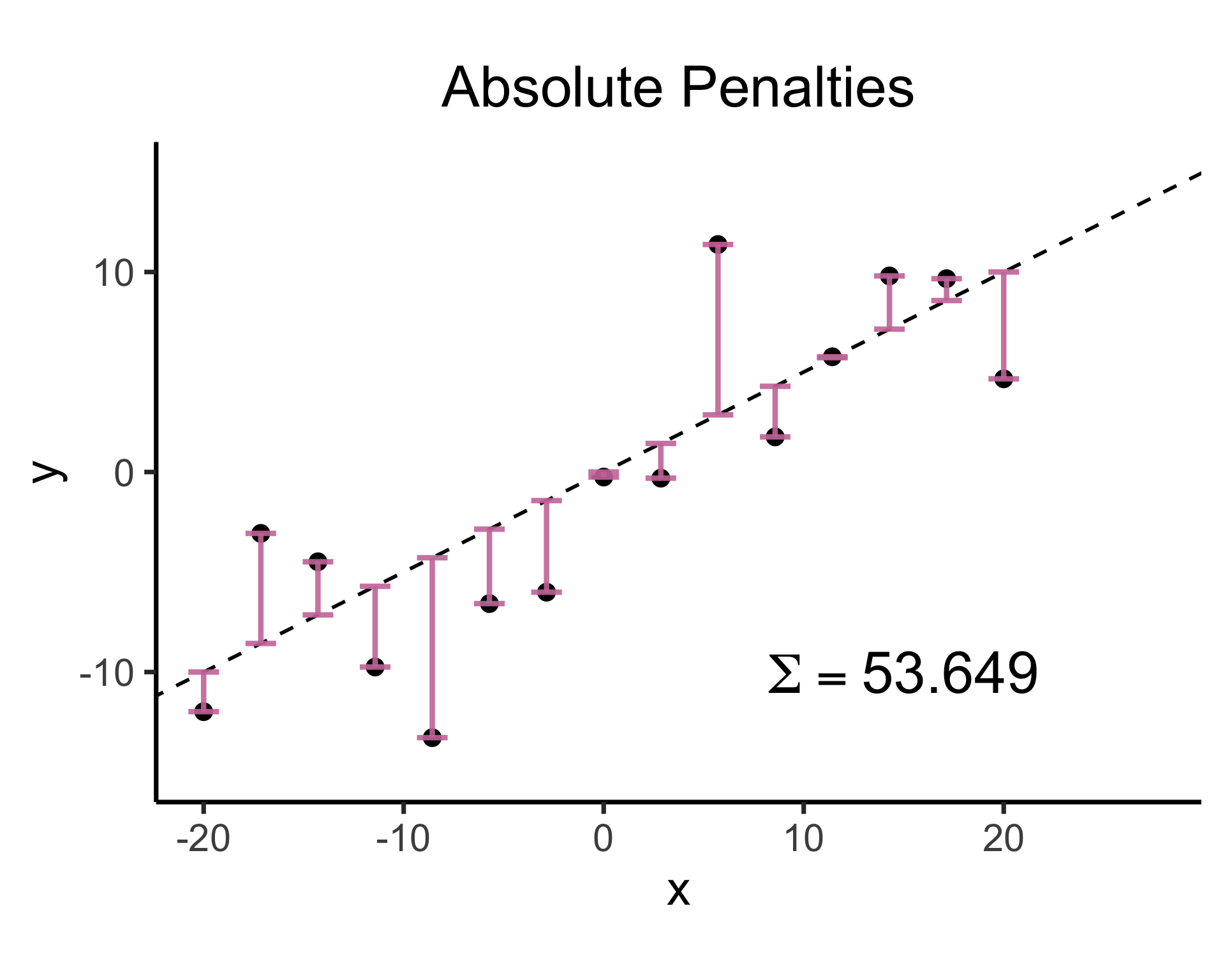
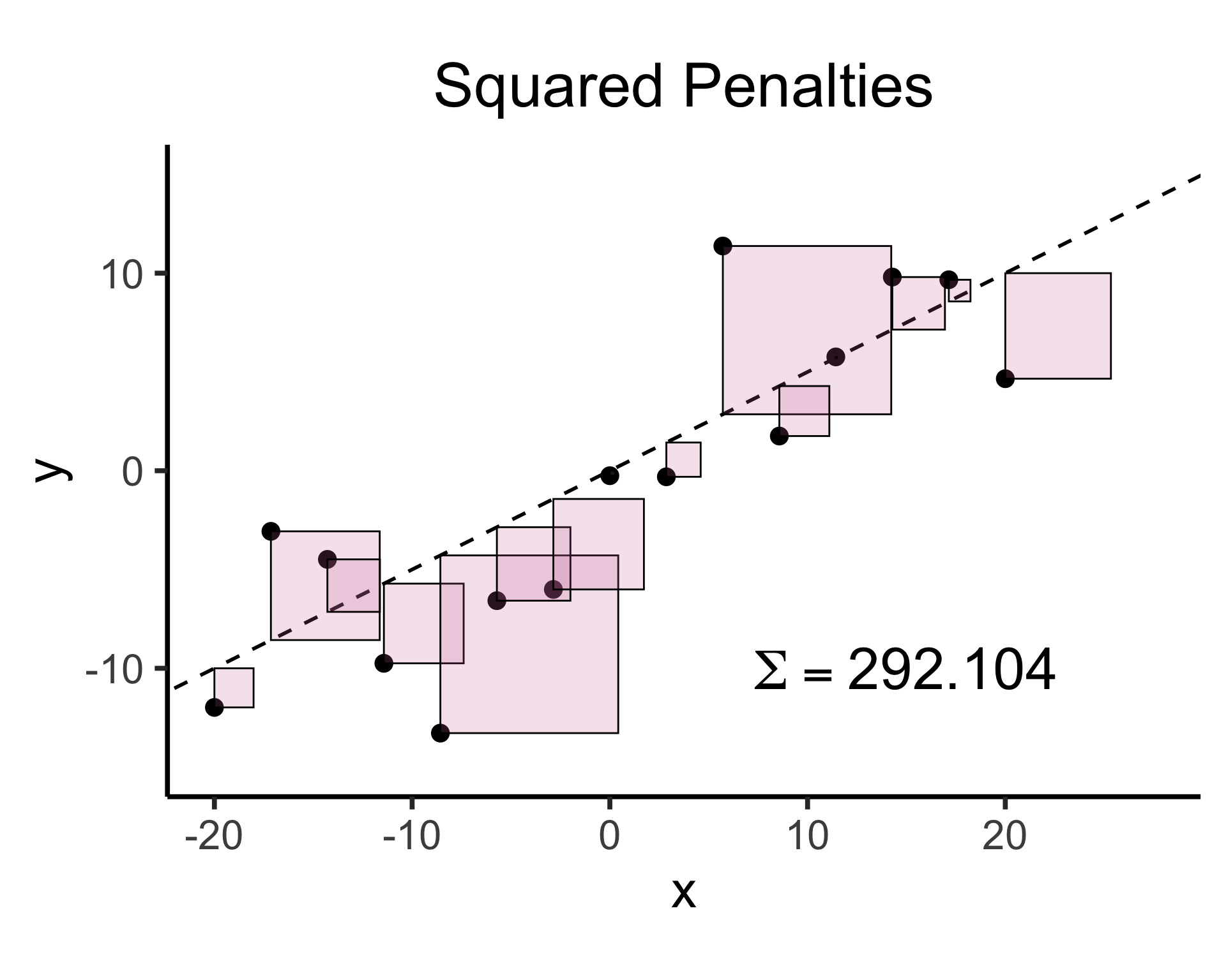
• Intuitively, two different ways to measure how well a line fits the data:

Figure 1: The line that minimizes blue distances does not predict \(Y\) as well as regression line, despite intuitive appeal!

Figure 2: The line that minimizes green distances optimally predicts \(Y\) from \(X\), in a mathematically-provable sense!

On the difference between these two lines, and why it matters, I cannot recommend Gelman and Hill (2007) enough!

Principal Component Analysis

• Principal Component Line can be used to project the data onto its dimension of highest variance (recap from 5000!)
• More simply: PCA can discover meaningful axes in data (unsupervised learning / exploratory data analysis settings)

See this amazing blog post using PCA, with 2 dimensions, to explore UN voting patterns!

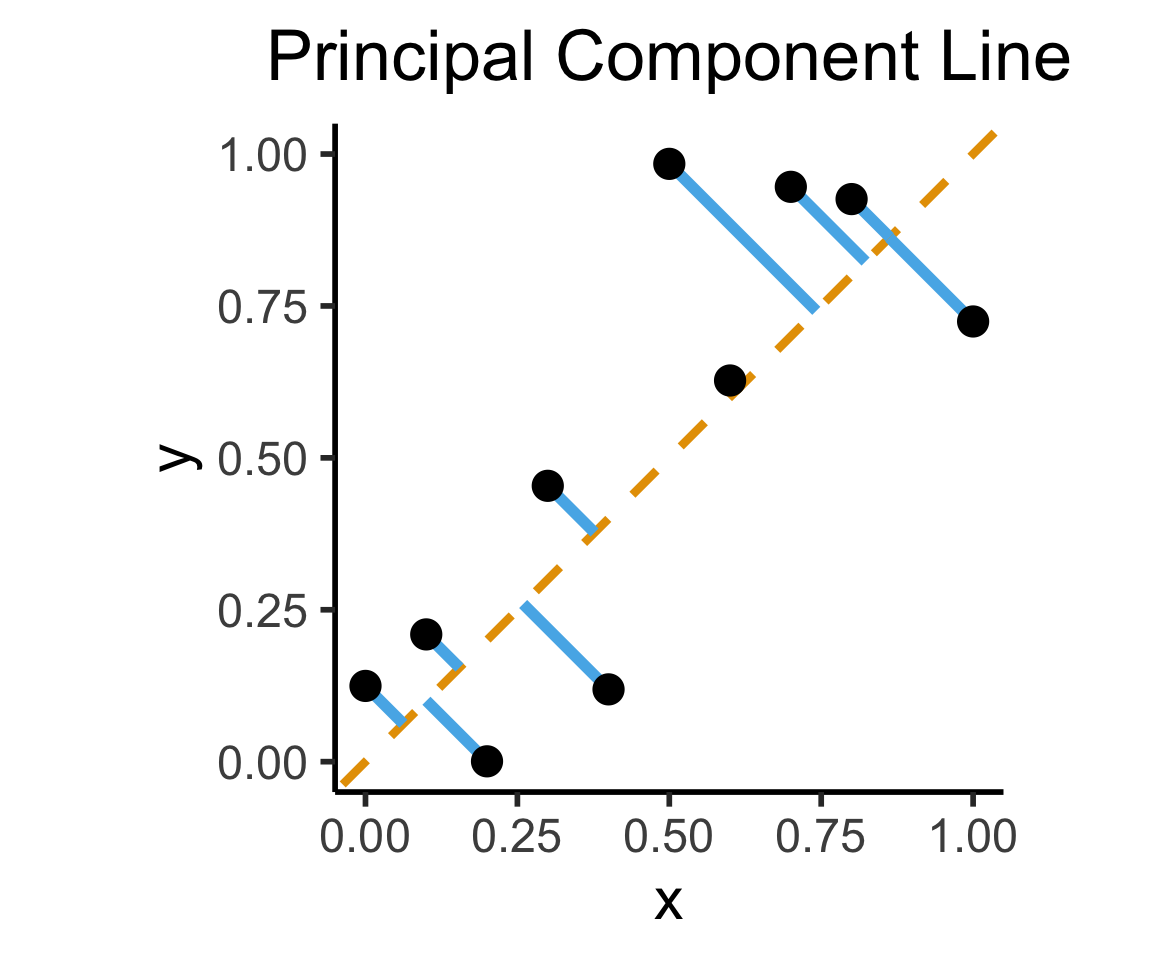
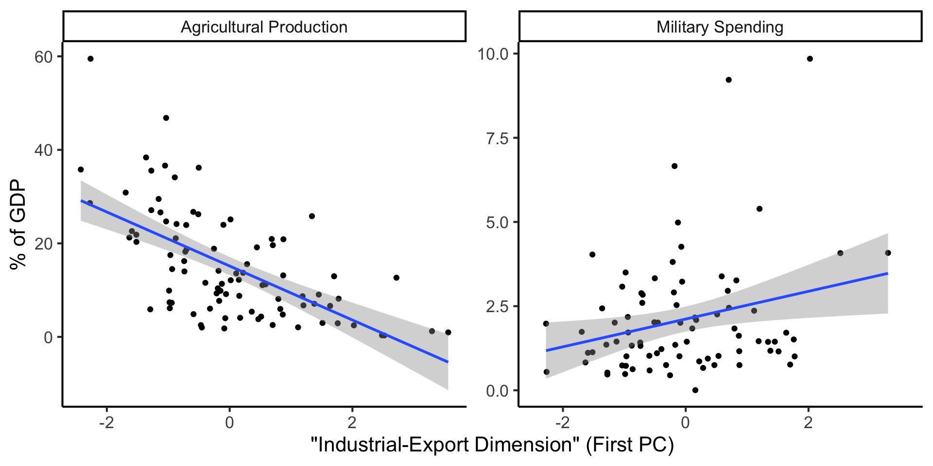
Create Your Own Dimension!

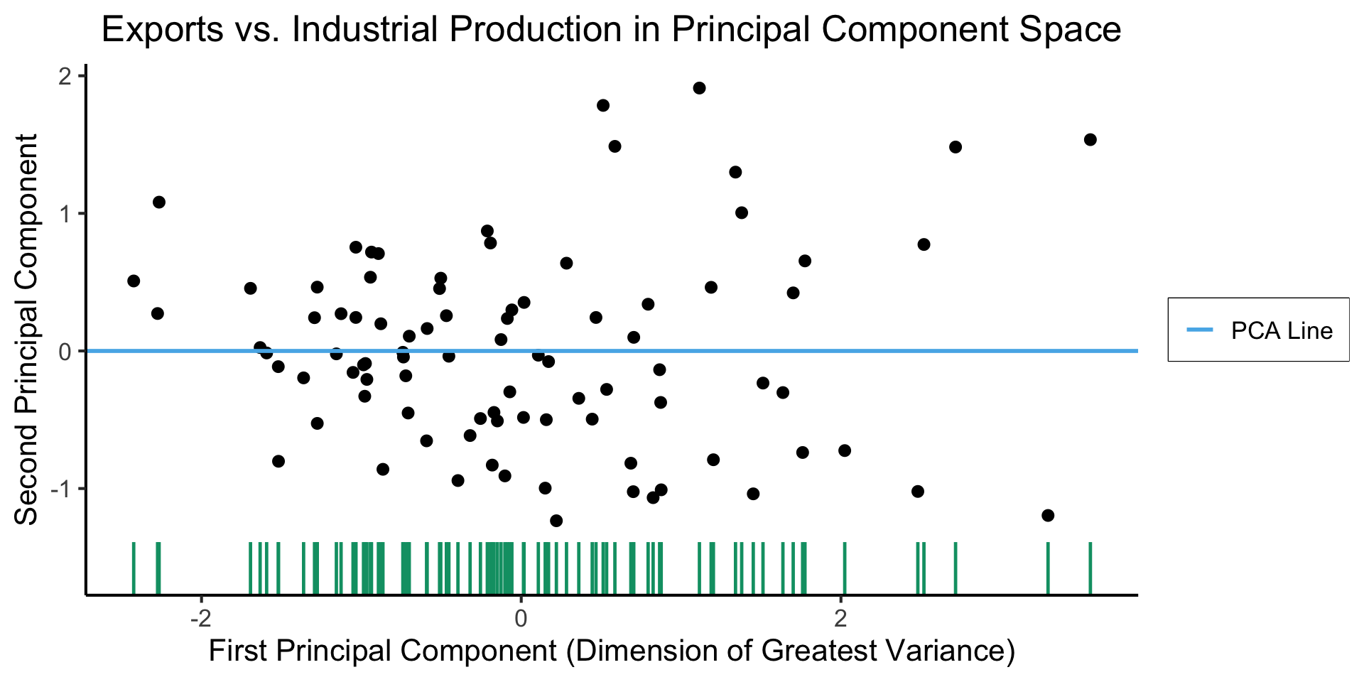
…And Use It for EDA

But in Our Case…

• \(x\) and \(y\) dimensions already have meaning, and we have a hypothesis about effect of \(x\) on \(y\)!

The Regression Hypothesis \(\mathcal{H}_{\text{reg}}\)

Given data \((X, Y)\), we estimate \(\widehat{y} = \widehat{\beta}_0 + \widehat{\beta}_1x\), hypothesizing that:

• Starting from \(y = \underbrace{\widehat{\beta}_0}_{\mathclap{\text{Intercept}}}\) when \(x = 0\),
• An increase of \(x\) by 1 unit is associated with an increase of \(y\) by \(\underbrace{\widehat{\beta}_1}_{\mathclap{\text{Coefficient}}}\) units

• We want to measure how well our line predicts \(y\) for any given \(x\) value \(\implies\) vertical distance from regression line

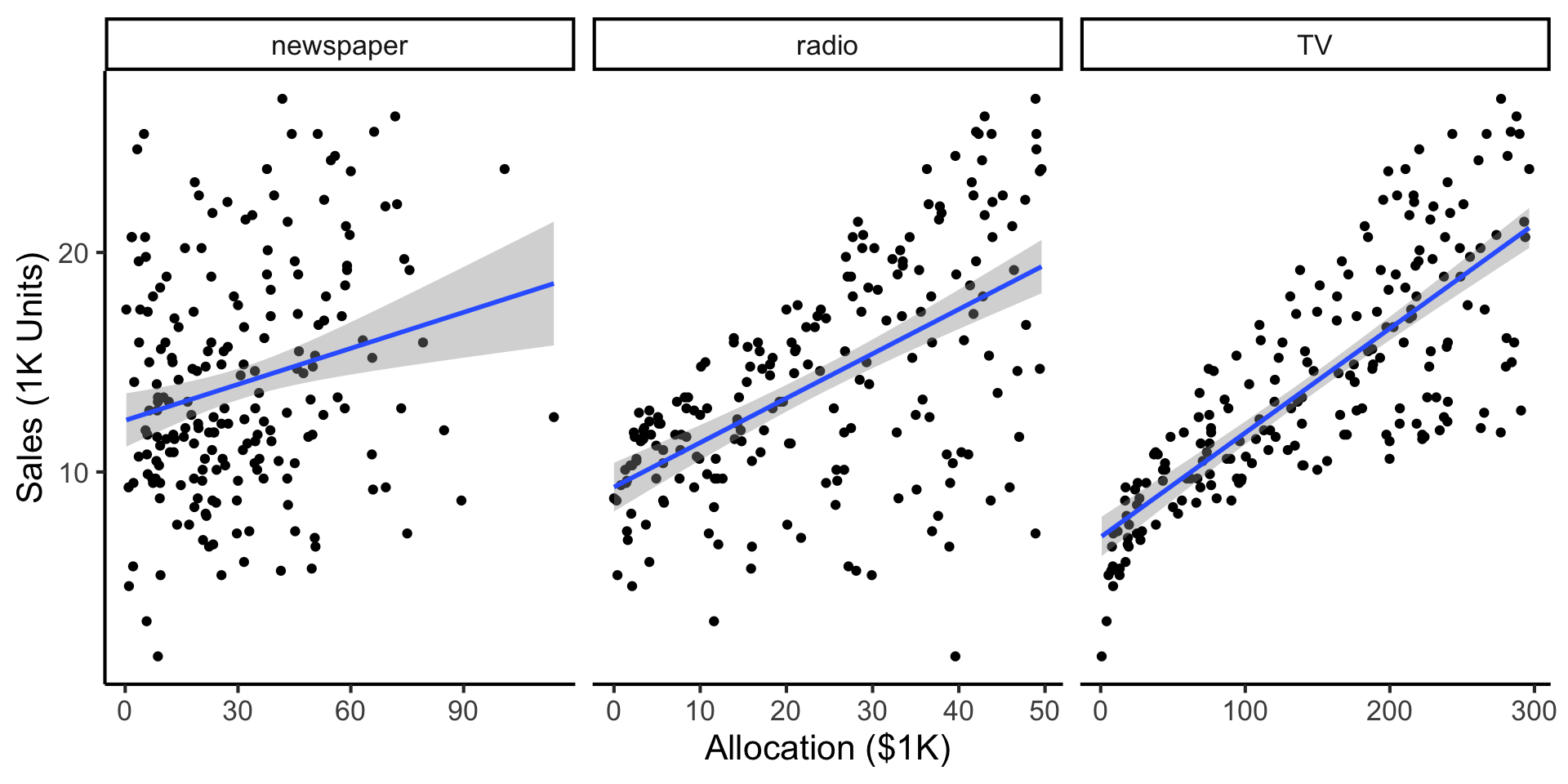
Example: Advertising Effects

• Independent variable: $ put into advertisements; Dependent variable: Sales
• Goal 1: Predict sales for a given allocation
• Goal 2: Infer best allocation for a given advertising budget (more simply: a new $1K appears! Where should we invest it?)

Simple Linear Regression

• For now, we treat Newspaper, Radio, TV advertising separately: how much do sales increase per $1 into [medium]? (Later we’ll consider them jointly: multiple regression)

Our model:

\[ Y = \underbrace{\param{\beta_0}}_{\mathclap{\text{Intercept}}} + \underbrace{\param{\beta_1}}_{\mathclap{\text{Slope}}}X + \varepsilon \]

…Generates predictions via:

\[ \widehat{y} = \underbrace{\widehat{\beta}_0}_{\mathclap{\small\begin{array}{c}\text{Estimated} \\[-5mm] \text{intercept}\end{array}}} ~+~ \underbrace{\widehat{\beta}_1}_{\mathclap{\small\begin{array}{c}\text{Estimated} \\[-4mm] \text{slope}\end{array}}}\cdot x \]

• Note how these predictions will be wrong (unless the data is perfectly linear)
• We’ve accounted for this in our model (by including \(\varepsilon\) term)!
• But, we’d like to find estimates \(\widehat{\beta}_0\) and \(\widehat{\beta}_1\) that produce the “least wrong” predictions: motivates focus on residuals \(\widehat{\varepsilon}_i\)…

\[ \widehat{\varepsilon}_i = \underbrace{y_i}_{\mathclap{\small\begin{array}{c}\text{Real} \\[-5mm] \text{label}\end{array}}} - \underbrace{\widehat{y}_i}_{\mathclap{\small\begin{array}{c}\text{Predicted} \\[-5mm] \text{label}\end{array}}} = \underbrace{y_i}_{\mathclap{\small\begin{array}{c}\text{Real} \\[-5mm] \text{label}\end{array}}} - \underbrace{ \left( \widehat{\beta}_0 + \widehat{\beta}_1 \cdot x \right) }_{\text{\small{Predicted label}}} \]

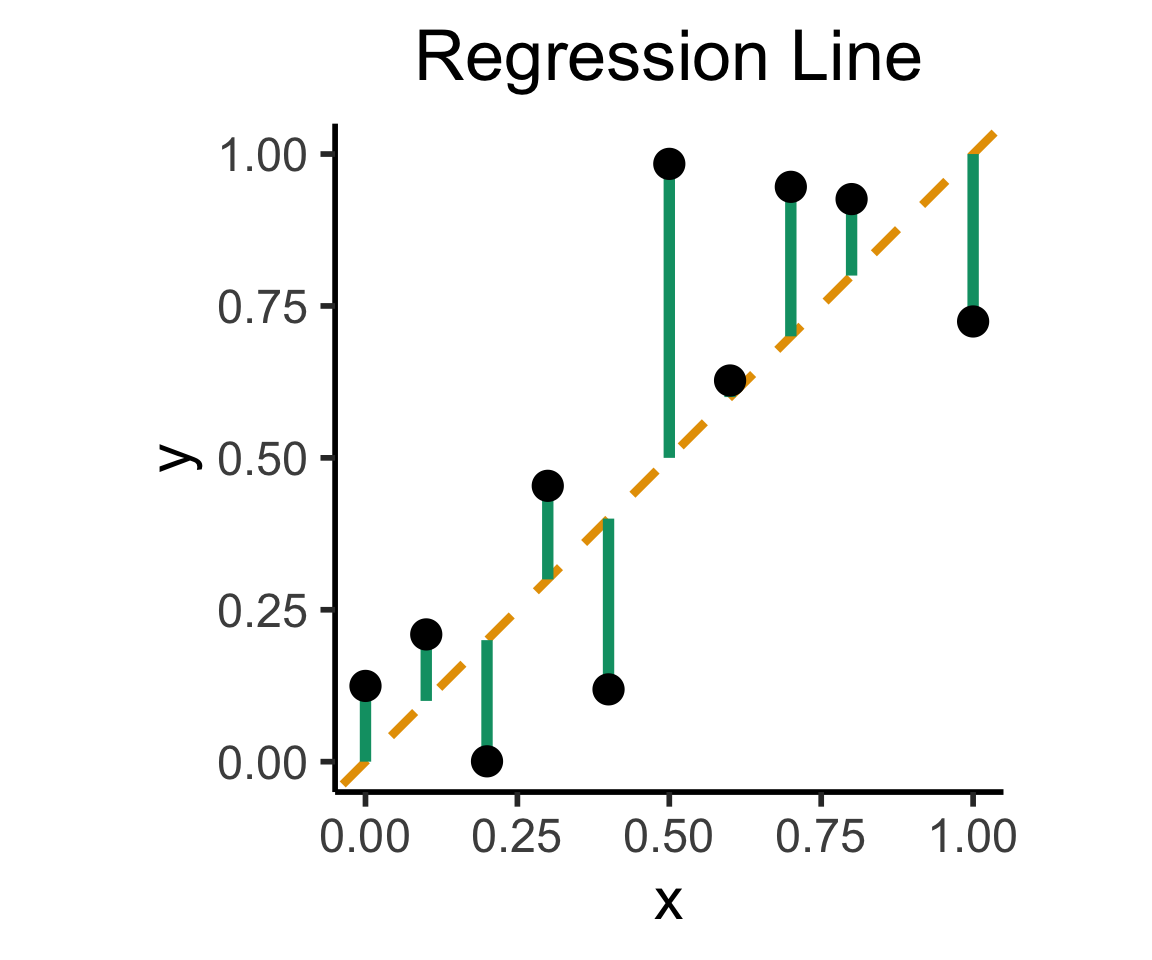
Least Squares: Minimizing Residuals

What can we optimize to ensure these residuals are as small as possible?

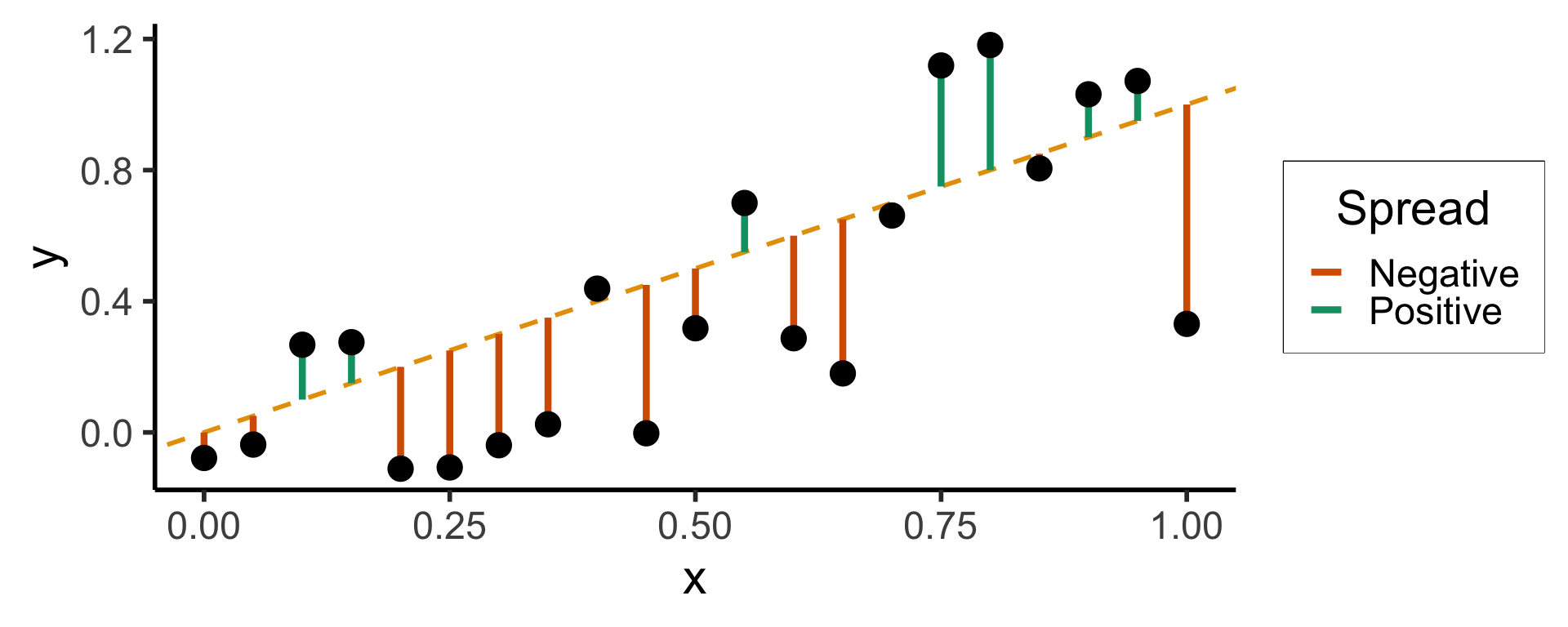
Sum?

0.0000000000

Sum of Squares?

3.8405017200

Sum of absolute vals?

7.6806094387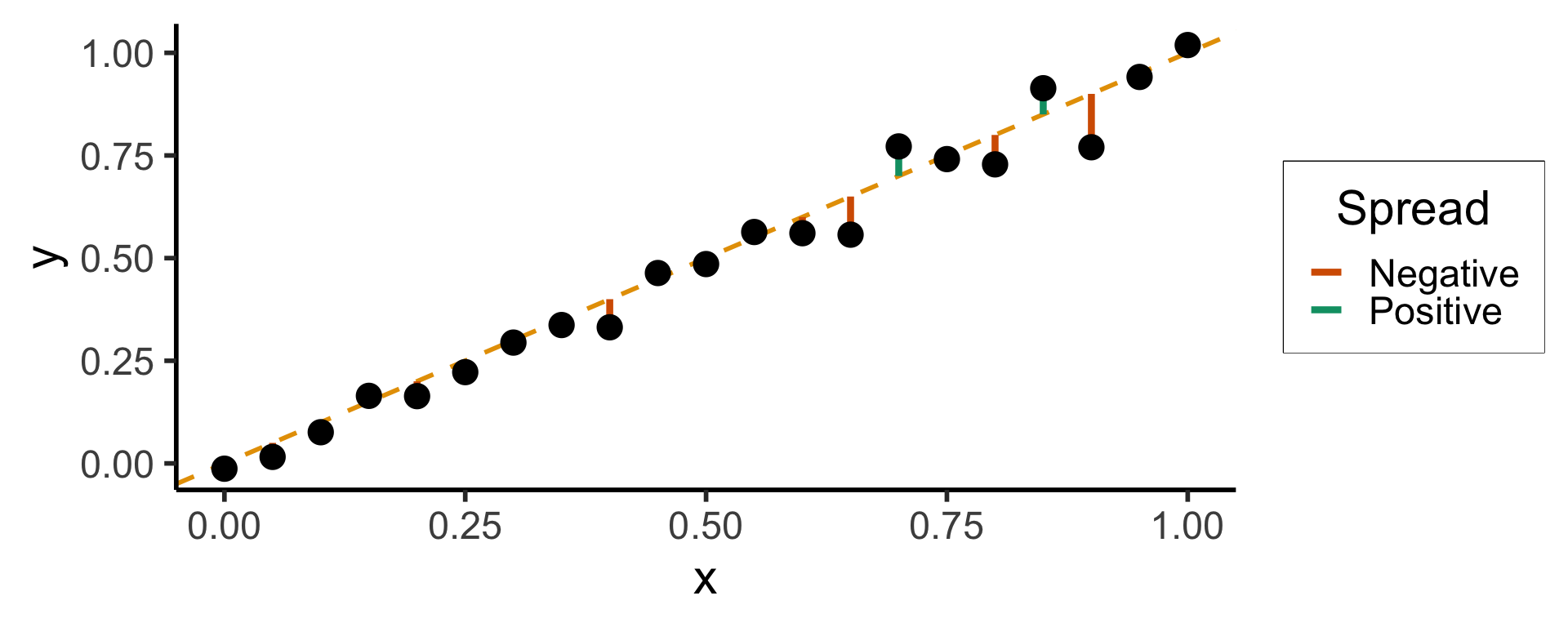

Sum?

0.0000000000

Sum of Squares?

1.9748635217

Sum of absolute vals?

5.5149697440

Why Not Absolute Value?

• Two feasible ways to prevent positive and negative residuals cancelling out:
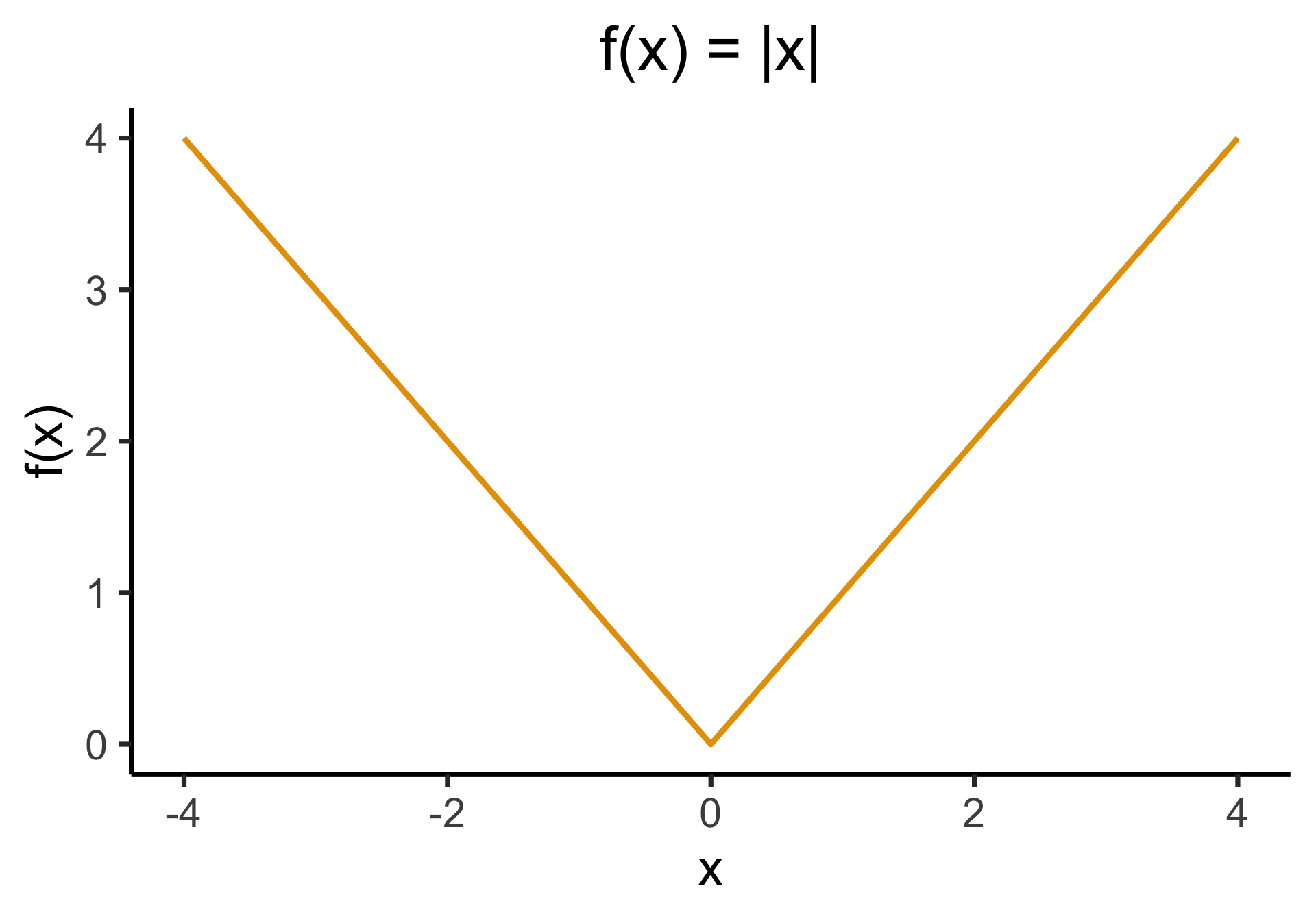
  • Absolute error \(\left|y - \widehat{y}\right|\) or squared error \(\left( y - \widehat{y} \right)^2\)
• But remember: we’re aiming to minimize 👀 these residuals; ghost of calculus past 😱
• We minimize by taking derivatives… which one is differentiable everywhere?

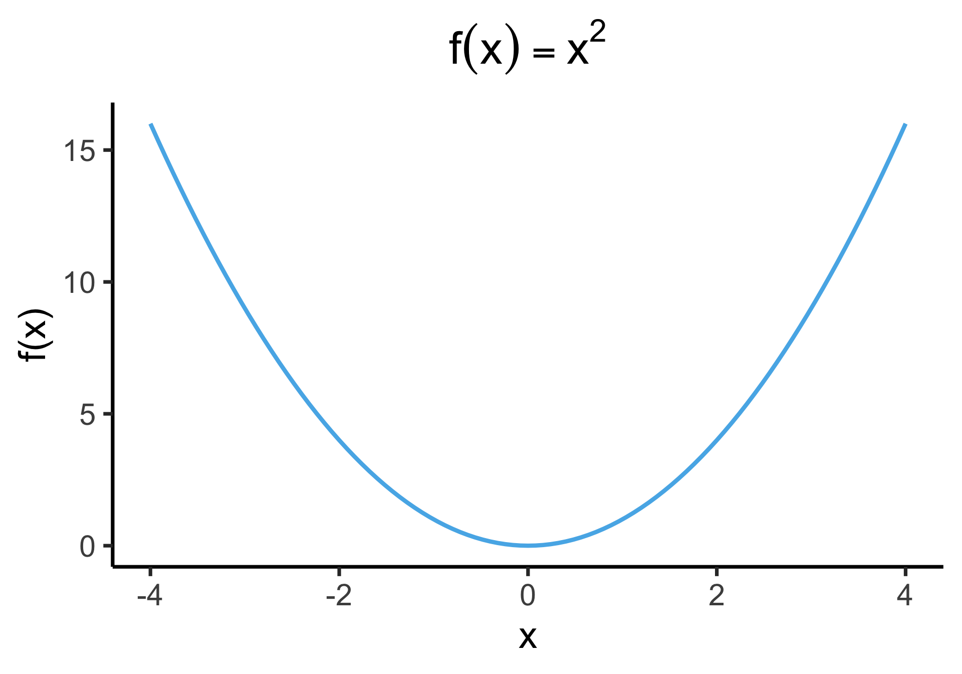
Outliers Penalized Quadratically

• May feel arbitrary at first (we’re “forced” to use squared error because of calculus?)
• It also has important consequences for “learnability” via gradient descent!

Key Features of Regression Line

• Regression line is BLUE: Best Linear Unbiased Estimator
• What exactly is it the “best” linear estimator of?

\[ \widehat{y} = \underbrace{\widehat{\beta}_0}_{\mathclap{\small\begin{array}{c}\text{Estimated} \\[-5mm] \text{intercept}\end{array}}} ~+~ \underbrace{\widehat{\beta}_1}_{\mathclap{\small\begin{array}{c}\text{Estimated} \\[-4mm] \text{slope}\end{array}}}\cdot x \]

is chosen so that

\[ \widehat{\theta} = \left(\widehat{\beta}_0, \widehat{\beta}_1\right) = \argmin_{\beta_0, \beta_1}\left[ \sum_{x_i \in X} \left(~~\overbrace{\widehat{y}(x_i)}^{\mathclap{\small\text{Predicted }y}} - \overbrace{\expect{Y \mid X = x_i}}^{\small \text{Avg. }y\text{ when }x = x_i}\right)^{2~} \right] \]

Where Did That \(\mathbb{E}[Y \mid X = x_i]\) Come From?

• From our assumption that the irreducible errors \(\varepsilon_i\) are normally distributed \(\mathcal{N}(0, \sigma^2)\)

Image Source

• Kind of an immensely important point, since it gives us a hint for checking whether model assumptions hold: spread around the regression line should be \(\mathcal{N}(0, \sigma^2)\)

Heteroskedasticity

• If spread increases or decreases for larger \(x\), for example, then \(\varepsilon \nsim \mathcal{N}(0, \sigma^2)\)

Figure 3.11 from James et al. (2023)

But… What About Other Types of Vars?

• 5000: you saw nominal, ordinal, cardinal vars
• 5100: you wrestled with discrete vs. continuous RVs
• Good News #1: Regression can handle all these types+more!
• Good News #2: Distinctions between classification and regression diminish as you learn fancier regression methods!
  • tldr: Predict continuous probabilities \(\Pr(Y) \in [0,1]\) (regression), then guess 1 if \(\Pr(Y) > 0.5\) (classification)
• By end of 5300 you should have something on your toolbelt for handling most cases like “I want to do [regression / classification], but my data is [not cardinal+continuous]”

Quiz Review

Objective Functions

“Fitting” a statistical model to data means minimizing some loss function that measures “how bad” our predictions are:

Optimization Problems: General Form

Find \(x^*\), the solution to

\[ \begin{align} \min_{x} ~ & f(x) &\text{(Objective function)} \\ \text{s.t. } ~ & g(x) = 0 &\text{(Constraints)} \end{align} \]

• Earlier we were able to write \(x^* = \argmax_x{f(x)}\), since there were no constraints. Is there a way to write a formula like this with constraints?
• Answer: Yes! Thx Giuseppe-Luigi Lagrangia = Joseph-Louis Lagrange:

\[ x^* = \argmax_{x,~\lambda}f(x) - \lambda[g(x)] \]

(Why worry about constraints when OLS is unconstrained? …Soon we’ll need to penalize complexity!)

Example Problem

Example 1: Unconstrained Optimization

Find \(x^*\), the solution to

\[ \begin{align} \min_{x} ~ & f(x) = 3x^2 - x \\ \text{s.t. } ~ & \varnothing \end{align} \]

Our Plan

• Compute the derivative \(f'(x) = \frac{\partial}{\partial x}f(x)\),
• Set it equal to zero: \(f'(x) = 0\), and
• Solve this equality for \(x\), i.e., find values \(x^*\) satisfying \(f'(x^*) = 0\)

Computing the derivative:

\[ f'(x) = \frac{\partial}{\partial x}f(x) = \frac{\partial}{\partial x}\left[3x^2 - x\right] = 6x - 1, \]

Solving for \(x^*\), the value(s) satisfying \(\frac{\partial}{\partial x}f'(x^*) = 0\) for just-derived \(f'(x)\):

\[ f'(x^*) = 0 \iff 6x^* - 1 = 0 \iff x^* = \frac{1}{6}. \]

Derivative Cheatsheet

Type of Thing	Thing	Change in Thing when \(x\) Changes by Tiny Amount
Polynomial	\(f(x) = x^n\)	\(f'(x) = \frac{\partial}{\partial x}f(x) = nx^{n-1}\)
Fraction	\(f(x) = \frac{1}{x}\)	Use Polynomial rule (since \(\frac{1}{x} = x^{-1}\)) to get \(f'(x) = -\frac{1}{x^2}\)
Logarithm	\(f(x) = \ln(x)\)	\(f'(x) = \frac{\partial}{\partial x} = \frac{1}{x}\)
Exponential	\(f(x) = e^x\)	\(f'(x) = \frac{\partial}{\partial x}e^x = e^x\) (🧐❗️)
Multiplication	\(f(x) = g(x)h(x)\)	\(f'(x) = g'(x)h(x) + g(x)h'(x)\)
Division	\(f(x) = \frac{g(x)}{h(x)}\)	Too hard to memorize… turn it into Multiplication, as \(f(x) = g(x)(h(x))^{-1}\)
Composition (Chain Rule)	\(f(x) = g(h(x))\)	\(f'(x) = g'(h(x))h'(x)\)
Fancy Logarithm	\(f(x) = \ln(g(x))\)	\(f'(x) = \frac{g'(x)}{g(x)}\) by Chain Rule
Fancy Exponential	\(f(x) = e^{g(x)}\)	\(f'(x) = g'(x)e^{g(x)}\) by Chain Rule

References

Gelman, Andrew, and Jennifer Hill. 2007. Data Analysis Using Regression and Multilevel/Hierarchical Models. Cambridge University Press. https://www.dropbox.com/scl/fi/asbumi3g0gqa4xl9va7wp/Andrew-Gelman-Jennifer-Hill-Data-Analysis-Using-Regression-and-Multilevel_Hierarchical-Models.pdf?rlkey=zf8icjhm7rswvxrpm7d10m65o&dl=1.

James, Gareth, Daniela Witten, Trevor Hastie, Robert Tibshirani, and Jonathan Taylor. 2023. An Introduction to Statistical Learning: With Applications in Python. Springer Nature. https://books.google.com?id=ygzJEAAAQBAJ.