Regression vs. PCA

DSAN 5300: Statistical Learning

Jeff Jacobs

jj1088@georgetown.edu

2025-02-03

The Central Tool of Data Science

\[ \DeclareMathOperator*{\argmax}{argmax} \DeclareMathOperator*{\argmin}{argmin} \newcommand{\bigexp}[1]{\exp\mkern-4mu\left[ #1 \right]} \newcommand{\bigexpect}[1]{\mathbb{E}\mkern-4mu \left[ #1 \right]} \newcommand{\definedas}{\overset{\small\text{def}}{=}} \newcommand{\definedalign}{\overset{\phantom{\text{defn}}}{=}} \newcommand{\eqeventual}{\overset{\text{eventually}}{=}} \newcommand{\Err}{\text{Err}} \newcommand{\expect}[1]{\mathbb{E}[#1]} \newcommand{\expectsq}[1]{\mathbb{E}^2[#1]} \newcommand{\fw}[1]{\texttt{#1}} \newcommand{\given}{\mid} \newcommand{\green}[1]{\color{green}{#1}} \newcommand{\heads}{\outcome{heads}} \newcommand{\iid}{\overset{\text{\small{iid}}}{\sim}} \newcommand{\lik}{\mathcal{L}} \newcommand{\loglik}{\ell} \DeclareMathOperator*{\maximize}{maximize} \DeclareMathOperator*{\minimize}{minimize} \newcommand{\mle}{\textsf{ML}} \newcommand{\nimplies}{\;\not\!\!\!\!\implies} \newcommand{\orange}[1]{\color{orange}{#1}} \newcommand{\outcome}[1]{\textsf{#1}} \newcommand{\param}[1]{{\color{purple} #1}} \newcommand{\pgsamplespace}{\{\green{1},\green{2},\green{3},\purp{4},\purp{5},\purp{6}\}} \newcommand{\prob}[1]{P\left( #1 \right)} \newcommand{\purp}[1]{\color{purple}{#1}} \newcommand{\sign}{\text{Sign}} \newcommand{\spacecap}{\; \cap \;} \newcommand{\spacewedge}{\; \wedge \;} \newcommand{\tails}{\outcome{tails}} \newcommand{\Var}[1]{\text{Var}[#1]} \newcommand{\bigVar}[1]{\text{Var}\mkern-4mu \left[ #1 \right]} \]

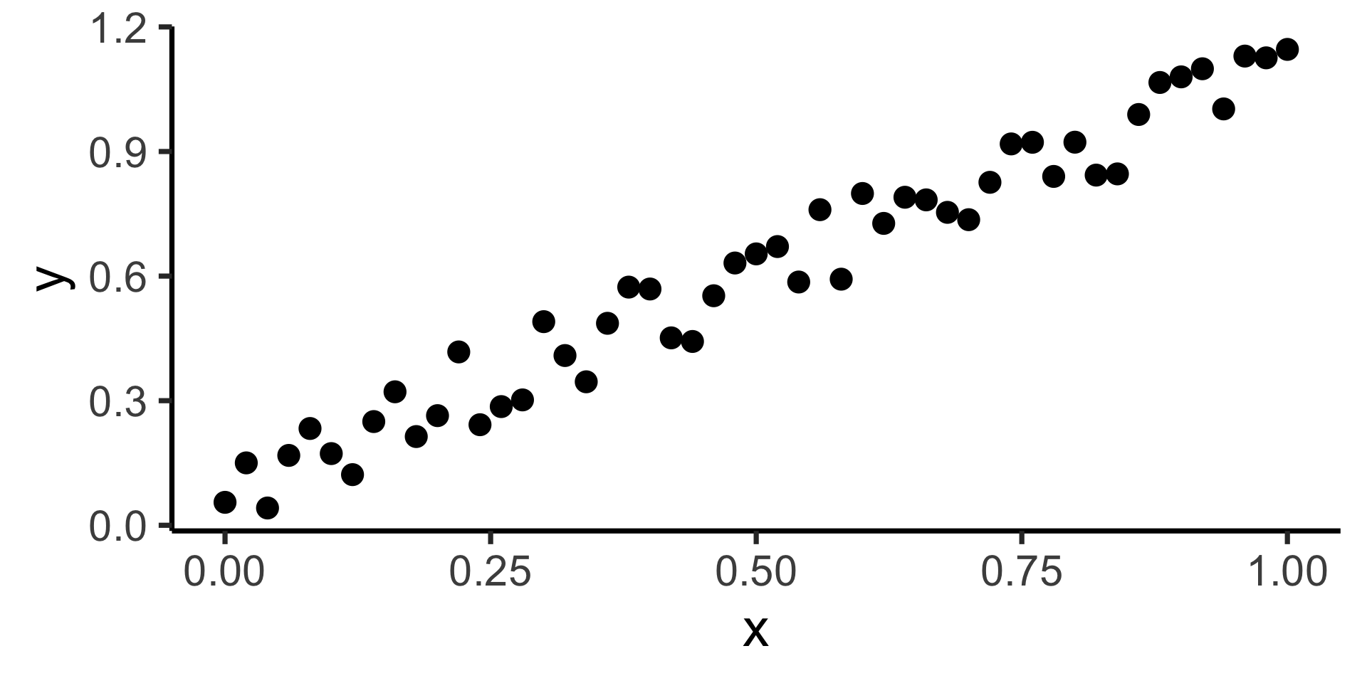
• If science is understanding relationships between variables, regression is the most basic but fundamental tool we have to start measuring these relationships
• Often exactly what humans do when we see data!

psychology psychology
trending_flat

The Goal

• Whenever you carry out a regression, keep the goal in the front of your mind:

The Goal of Regression

Find a line \(\widehat{y} = mx + b\) that best predicts \(Y\) for given values of \(X\)

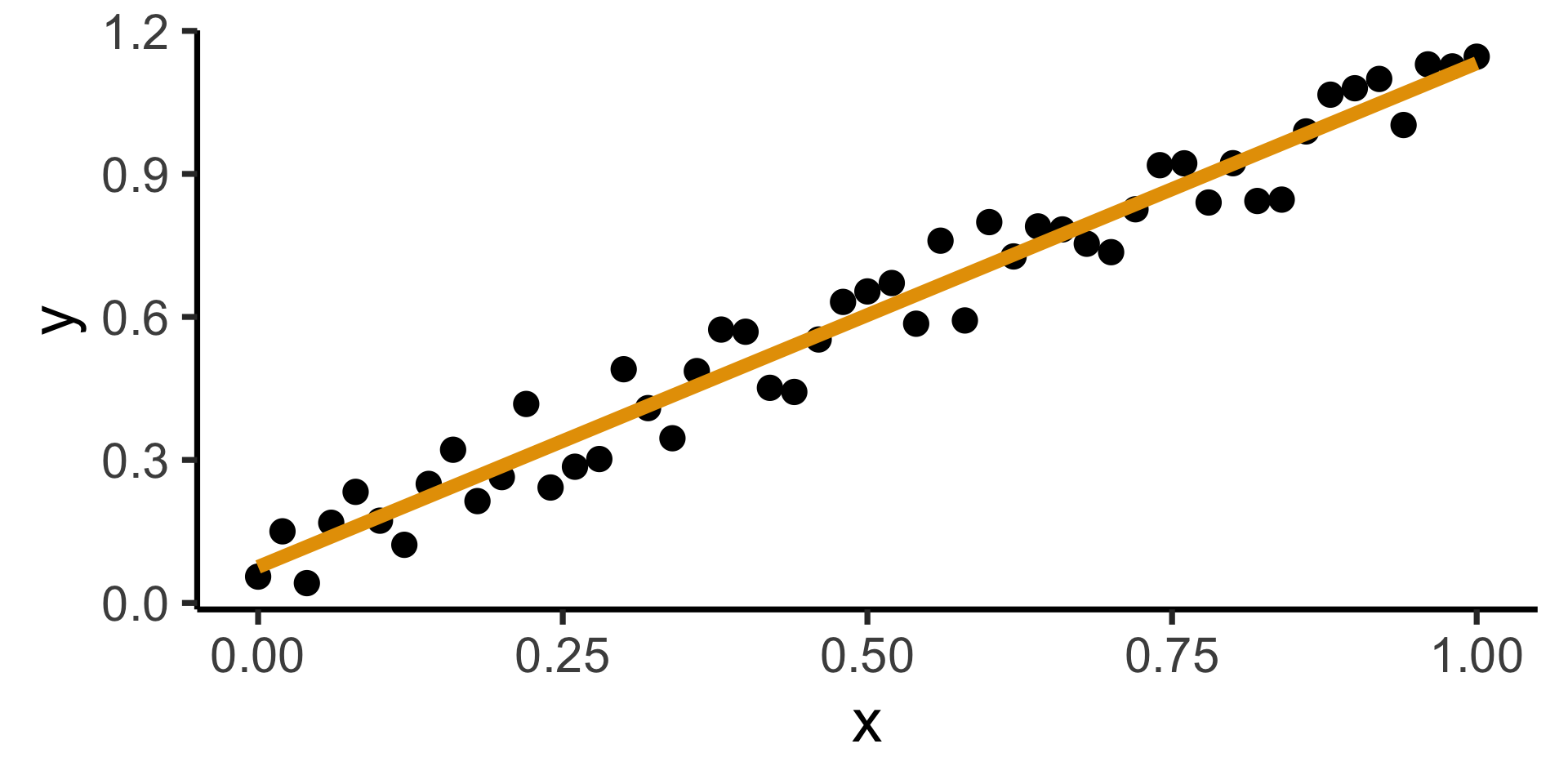
How Do We Define “Best”?

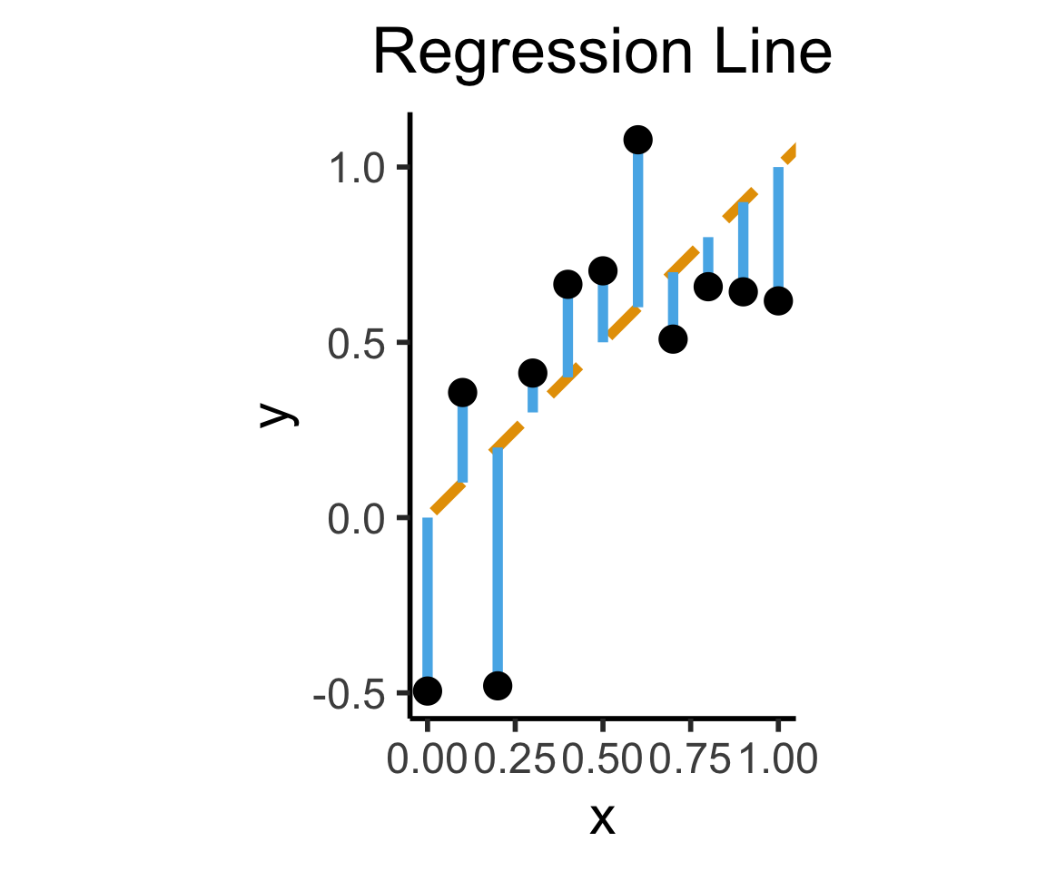
• Intuitively, two different ways to measure how well a line fits the data:

On the difference between these two lines, and why it matters, I cannot recommend Gelman and Hill (2007) enough!

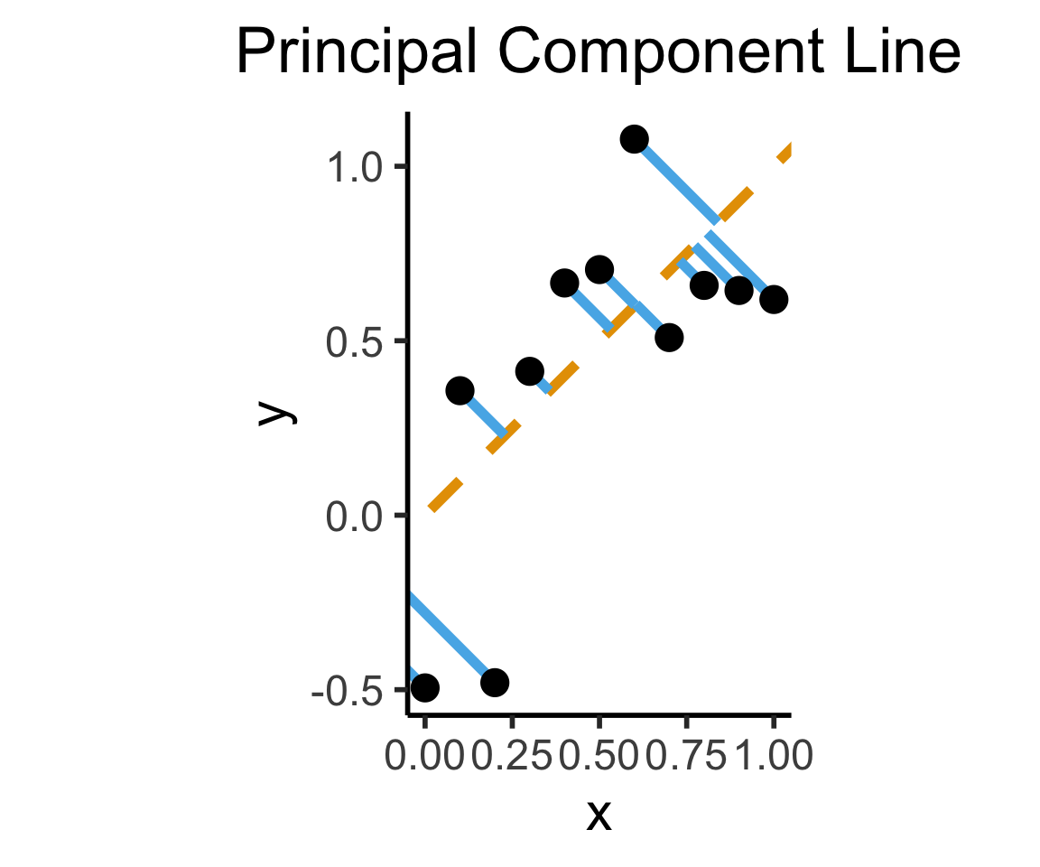
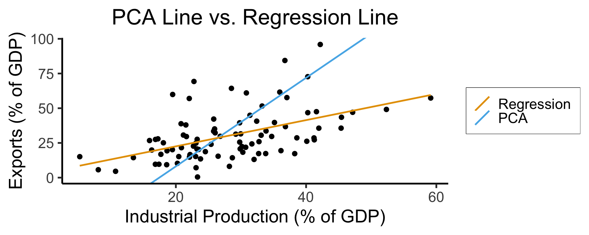
Principal Component Analysis

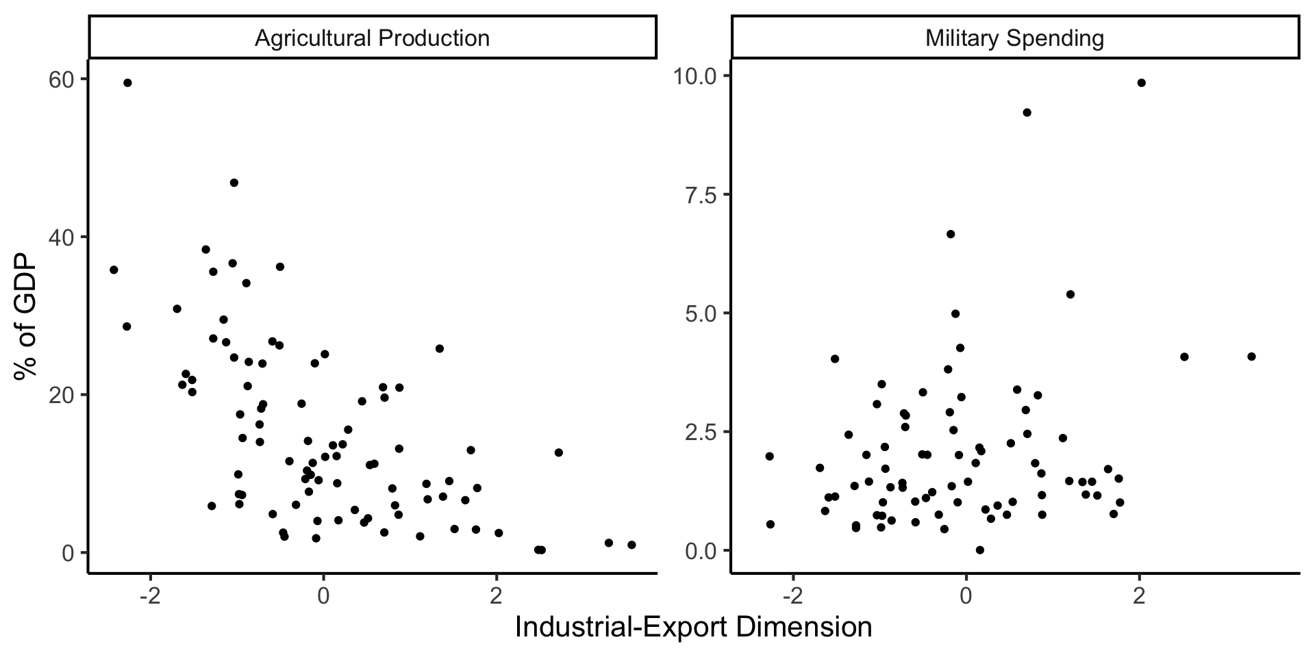
• Principal Component Line can be used to project the data onto its dimension of highest variance

• More simply: PCA can discover meaningful axes in data (unsupervised learning / exploratory data analysis settings)

See https://juliasilge.com/blog/un-voting/ for an amazing blog post using PCA, with 2 dimensions, to explore UN voting patterns!

Create Your Own Dimension!

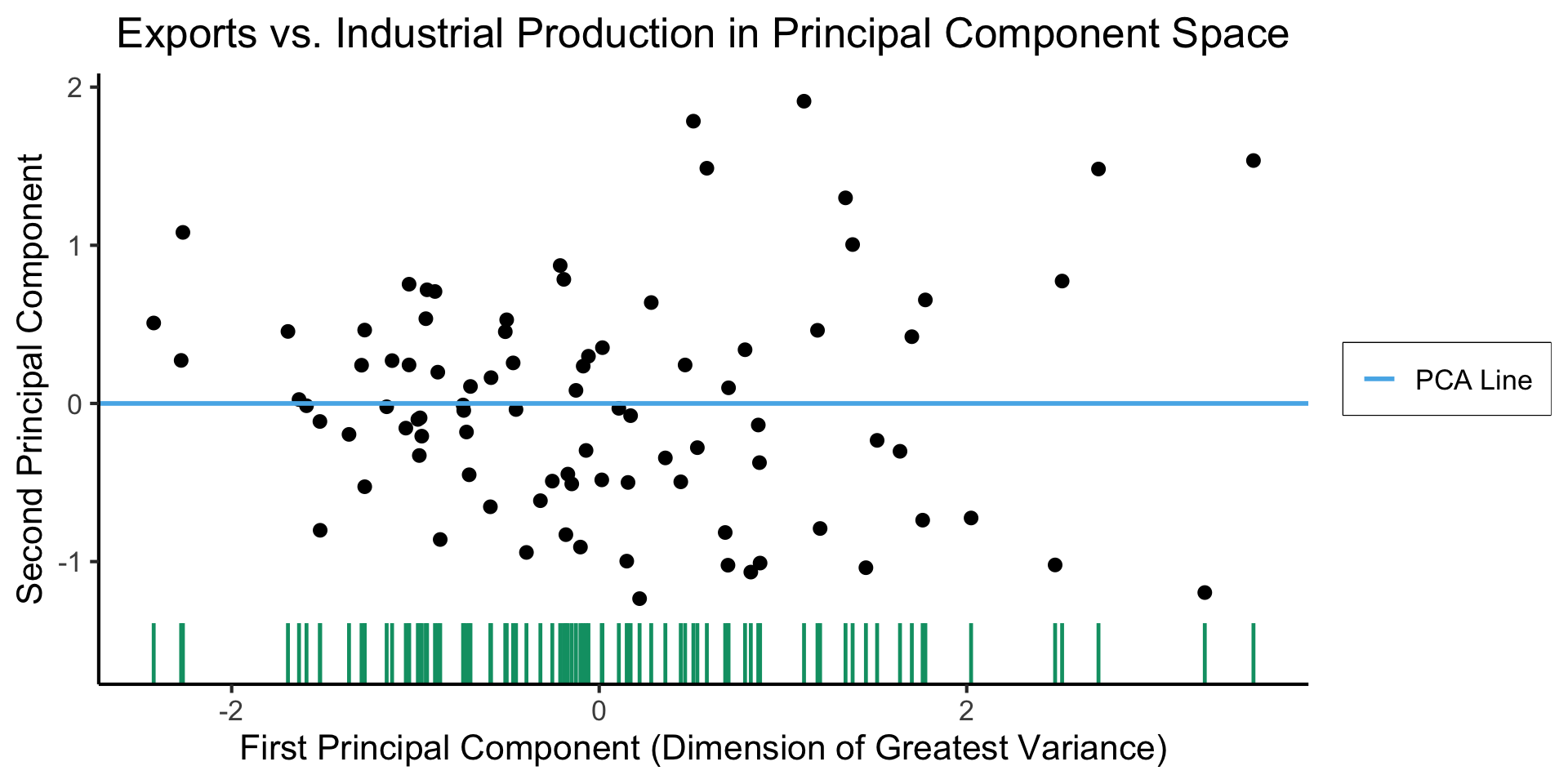
And Use It for EDA

But in Our Case…

• \(x\) and \(y\) dimensions already have meaning, and we have a hypothesis about \(x \rightarrow y\)!

The Regression Hypothesis \(\mathcal{H}_{\text{reg}}\)

Given data \((X, Y)\), we estimate \(\widehat{y} = \widehat{\beta_0} + \widehat{\beta_1}x\), hypothesizing that:

• Starting from \(y = \widehat{\beta_0}\) when \(x = 0\) (the intercept),
• An increase of \(x\) by 1 unit is associated with an increase of \(y\) by \(\widehat{\beta_1}\) units (the coefficient)

• We want to measure how well our line predicts \(y\) for any given \(x\) value \(\implies\) vertical distance from regression line

Key Features of Regression Line

• Regression line is BLUE: Best Linear Unbiased Estimator
• What exactly is it the “best” linear estimator of?

\[ \widehat{y} = \underbrace{\widehat{\beta_0}}_{\small\begin{array}{c}\text{Predicted} \\[-5mm] \text{intercept}\end{array}} + \underbrace{\widehat{\beta_1}}_{\small\begin{array}{c}\text{Predicted} \\[-4mm] \text{slope}\end{array}}\cdot x \]

is chosen so that

\[ \theta = \left(\widehat{\beta_0}, \widehat{\beta_1}\right) = \argmin_{\beta_0, \beta_1}\left[ \sum_{x_i \in X} \left(\overbrace{\widehat{y}(x_i)}^{\small\text{Predicted }y} - \overbrace{\expect{Y \mid X = x_i}}^{\small \text{Avg. }y\text{ when }x = x_i}\right)^2 \right] \]

Regression in R

lin_model <- lm(military ~ industrial, data=gdp_df)
summary(lin_model)

Call:
lm(formula = military ~ industrial, data = gdp_df)

Residuals:
    Min      1Q  Median      3Q     Max 
-2.3354 -1.0997 -0.3870  0.6081  6.7508 

Coefficients:
            Estimate Std. Error t value Pr(>|t|)  
(Intercept)  0.61969    0.59526   1.041   0.3010  
industrial   0.05253    0.02019   2.602   0.0111 *
---
Signif. codes:  0 '***' 0.001 '**' 0.01 '*' 0.05 '.' 0.1 ' ' 1

Residual standard error: 1.671 on 79 degrees of freedom
  (8 observations deleted due to missingness)
Multiple R-squared:  0.07895,   Adjusted R-squared:  0.06729 
F-statistic: 6.771 on 1 and 79 DF,  p-value: 0.01106

lm Syntax

lm(
  formula = dependent ~ independent + controls,
  data = my_df
)

Interpreting Output

Call:
lm(formula = military ~ industrial, data = gdp_df)

Residuals:
    Min      1Q  Median      3Q     Max 
-2.3354 -1.0997 -0.3870  0.6081  6.7508 

Coefficients:
            Estimate Std. Error t value Pr(>|t|)  
(Intercept)  0.61969    0.59526   1.041   0.3010  
industrial   0.05253    0.02019   2.602   0.0111 *

---
Signif. codes:  0 '***' 0.001 '**' 0.01 '*' 0.05 '.' 0.1 ' ' 1
Residual standard error: 1.671 on 79 degrees of freedom
  (8 observations deleted due to missingness)
Multiple R-squared:  0.07895,   Adjusted R-squared:  0.06729 
F-statistic: 6.771 on 1 and 79 DF,  p-value: 0.01106

Zooming In: Coefficients

	Estimate	Std. Error	t value	Pr(>|t|)
(Intercept)	0.61969	0.59526	1.041	0.3010
industrial	0.05253	0.02019	2.602	0.0111	*
	\(\widehat{\beta}\)	Uncertainty	Test statistic	How extreme is test stat?	Statistical significance

\[ \widehat{y} \approx \class{cb1}{\overset{\beta_0}{\underset{\small \pm 0.595}{0.620}}} + \class{cb2}{\overset{\beta_1}{\underset{\small \pm 0.020}{0.053}}} \cdot x \]

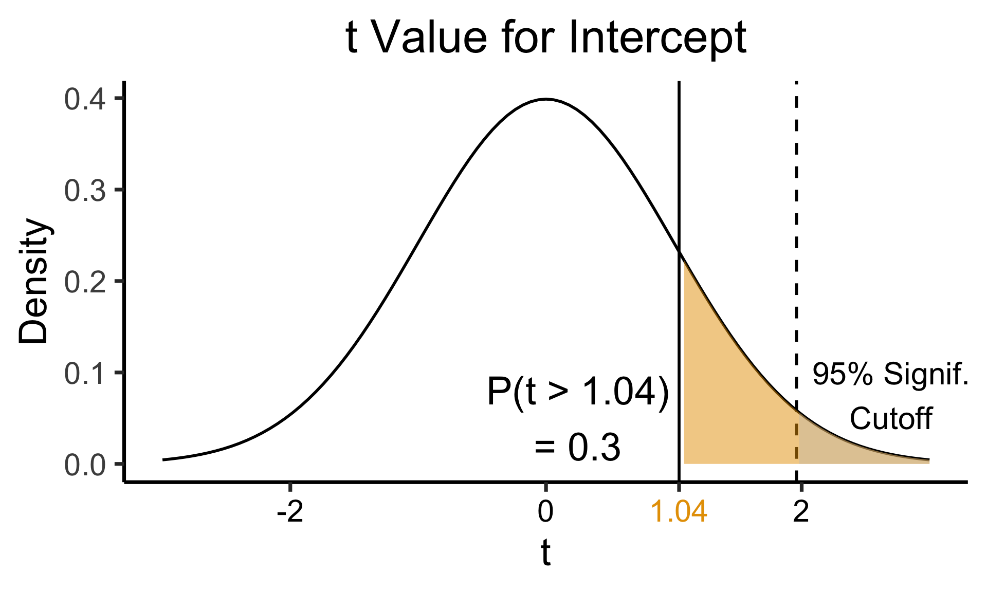
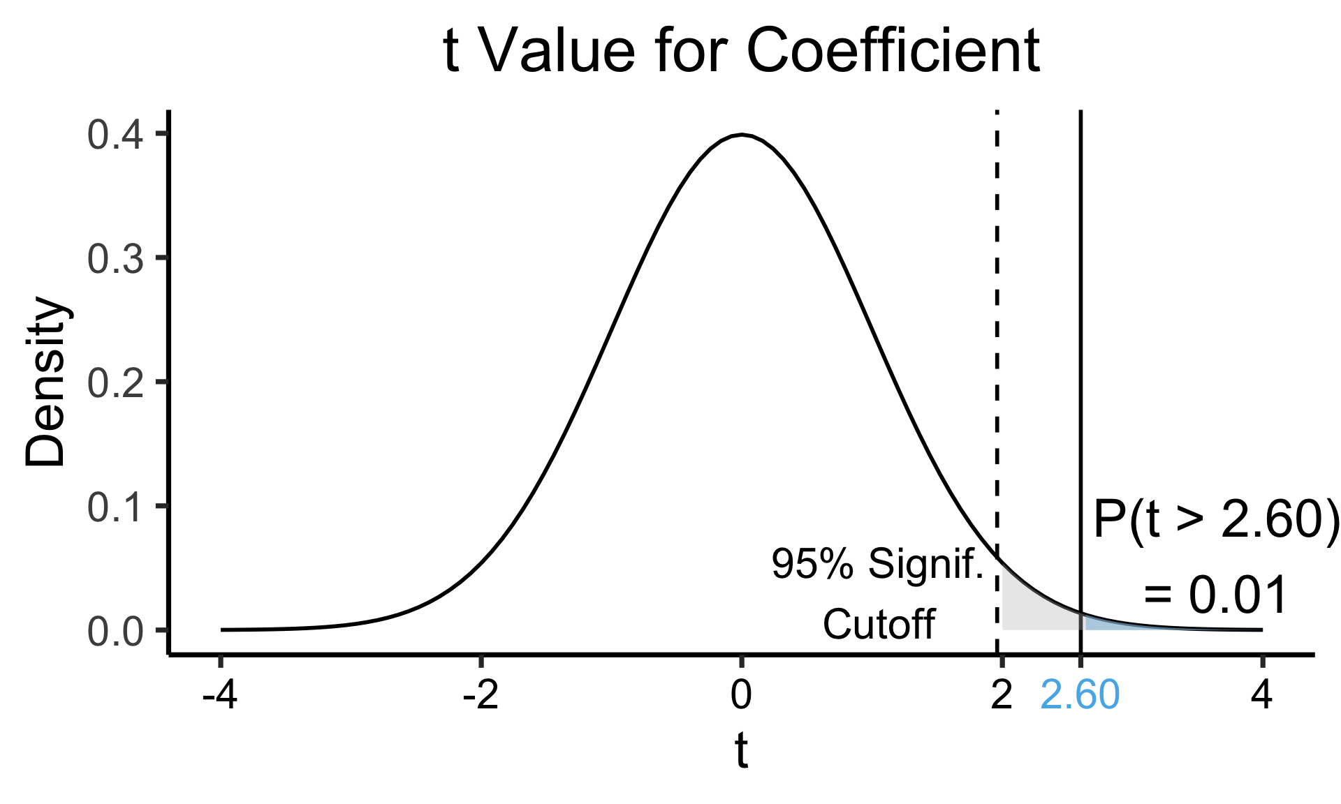
Zooming In: Significance

	Estimate	Std. Error	t value	Pr(>|t|)
(Intercept)	0.61969	0.59526	1.041	0.3010
industrial	0.05253	0.02019	2.602	0.0111	*
	\(\widehat{\beta}\)	Uncertainty	Test statistic	How extreme is test stat?	Statistical significance

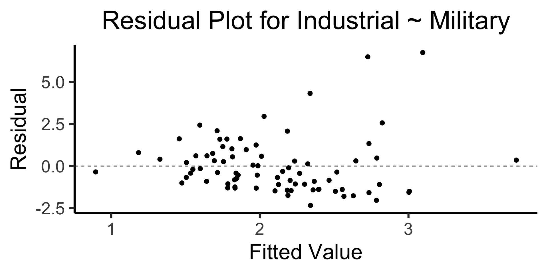
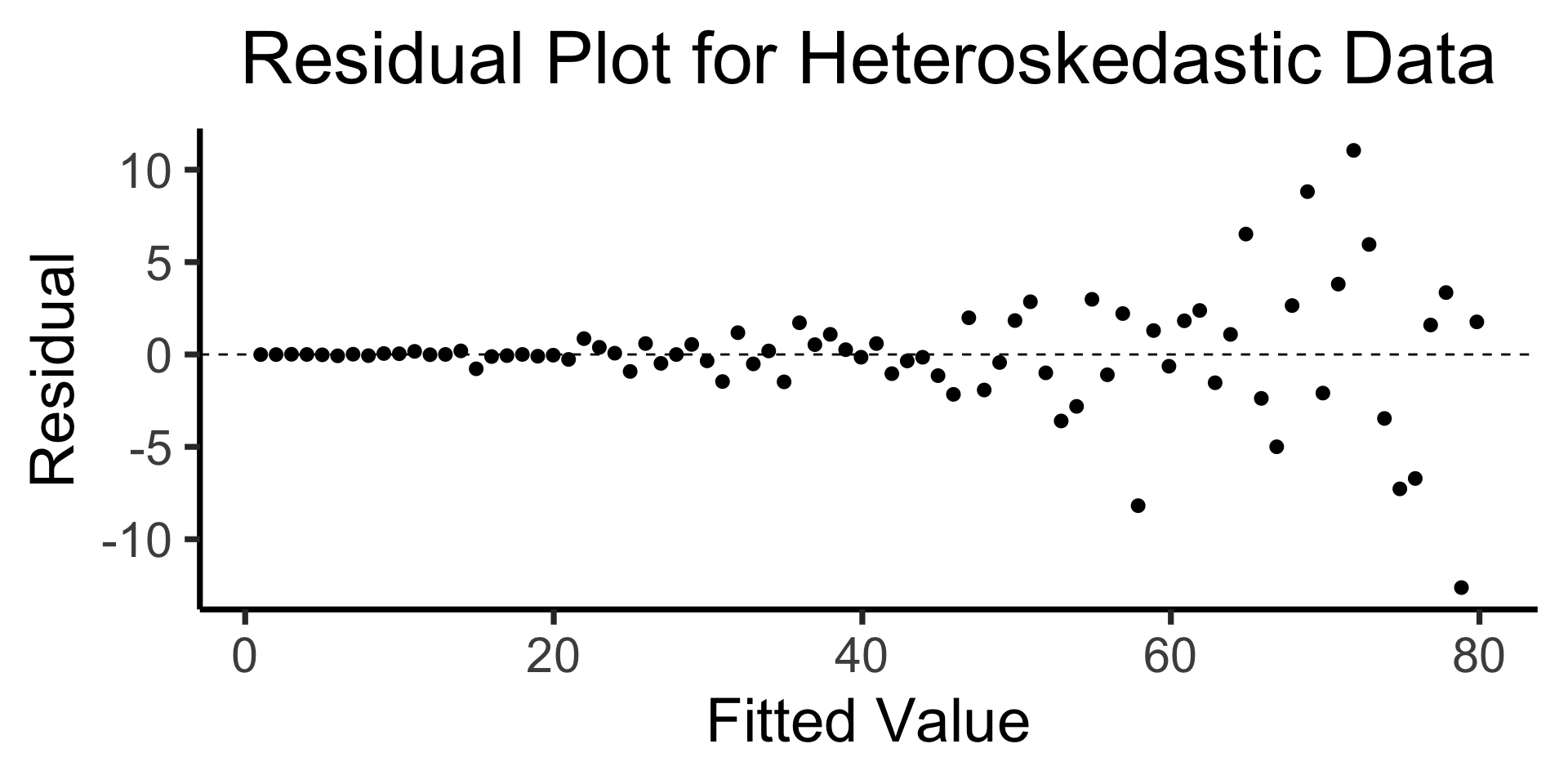
The Residual Plot

• A key assumption required for OLS: “homoskedasticity”
• Given our model \[ y_i = \beta_0 + \beta_1x_i + \varepsilon_i \] the errors \(\varepsilon_i\) should not vary systematically with \(i\)
• Formally: \(\forall i \left[ \Var{\varepsilon_i} = \sigma^2 \right]\)

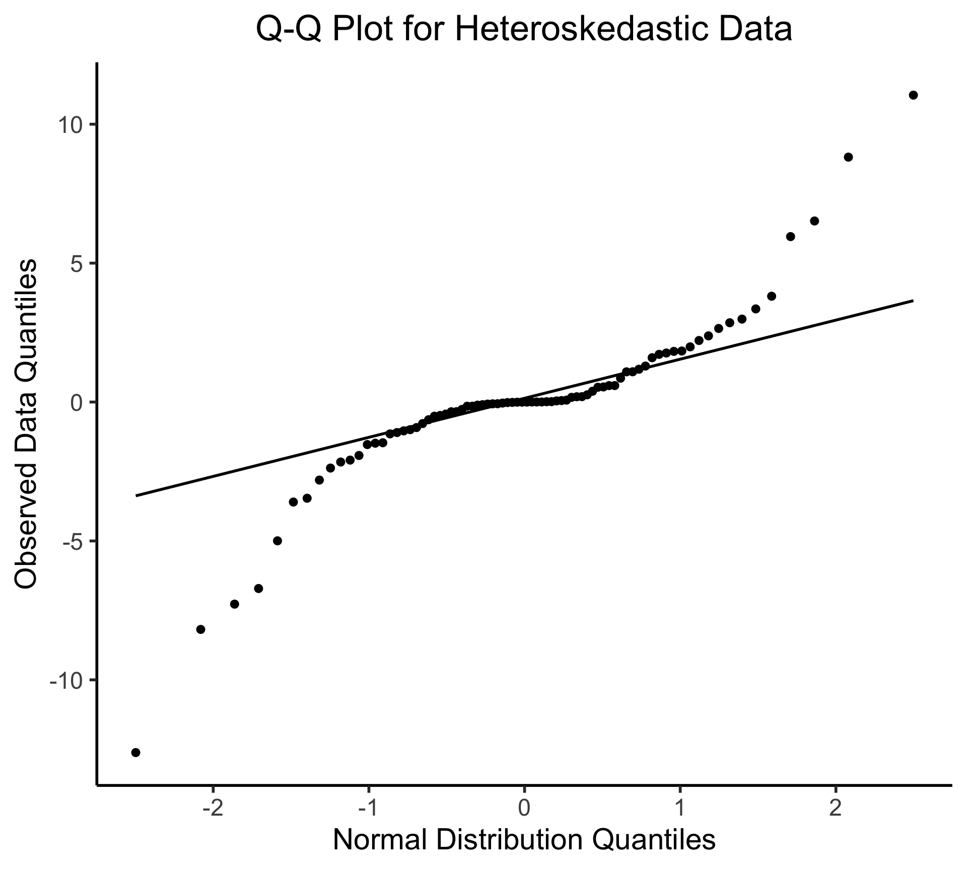
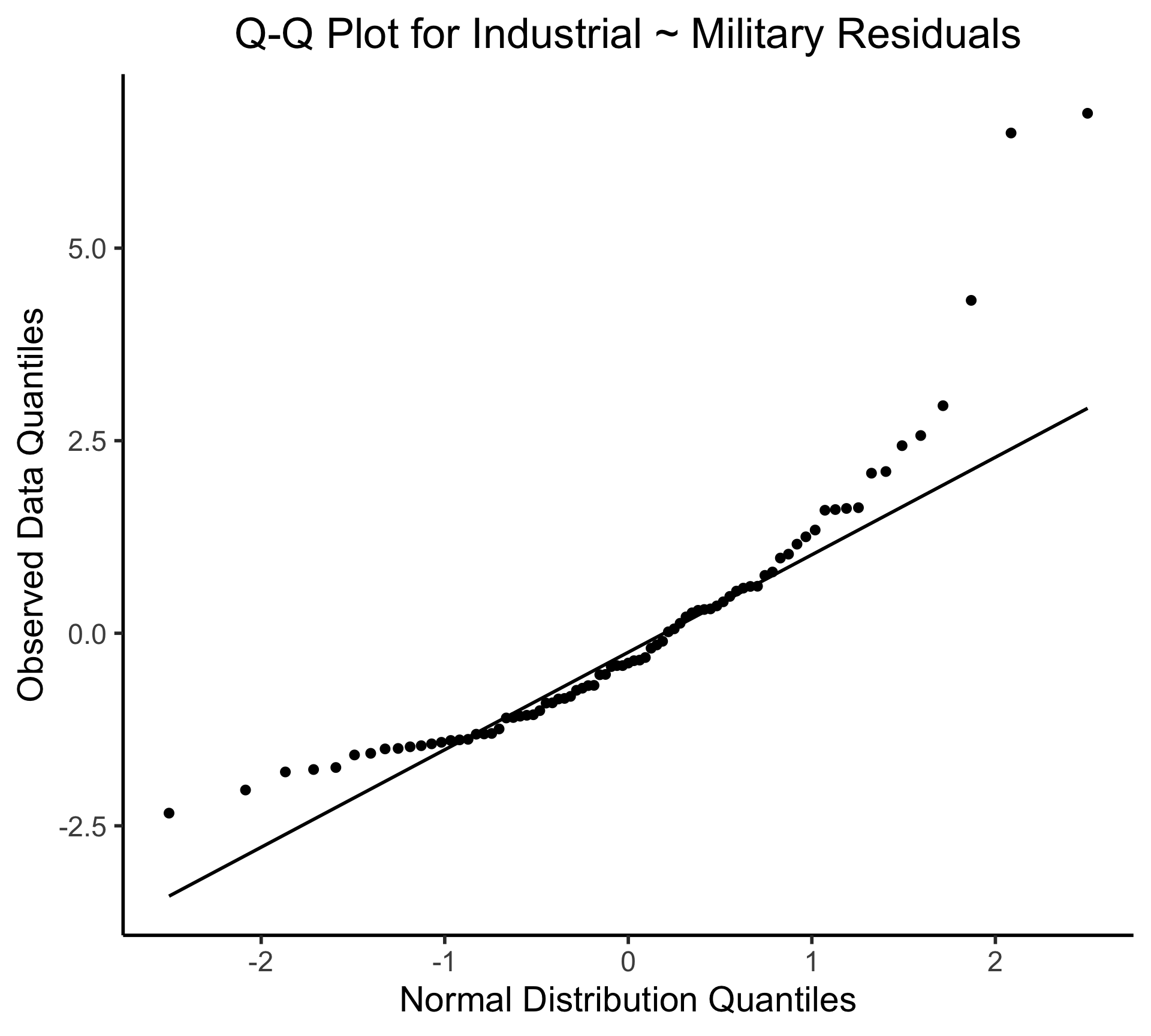
Q-Q Plot

• If \((\widehat{y} - y) \sim \mathcal{N}(0, \sigma^2)\), points would lie on 45° line:

Multiple Linear Regression

• Notation: \(x_{i,j}\) = value of independent variable \(j\) for person/observation \(i\)
• \(M\) = total number of independent variables

\[ \widehat{y}_i = \beta_0 + \beta_1x_{i,1} + \beta_2x_{i,2} + \cdots + \beta_M x_{i,M} \]

• \(\beta_j\) interpretation: a one-unit increase in \(x_{i,j}\) is associated with a \(\beta_j\) unit increase in \(y_i\), holding all other independent variables constant

References

Gelman, Andrew, and Jennifer Hill. 2007. Data Analysis Using Regression and Multilevel/Hierarchical Models. Cambridge University Press.