Extra Slides: A Slightly Deeper Dive Into Machine Learning

DSAN5000: Data Science and Analytics
(Addendum to Week 07)

Author

Affiliation

Jeff Jacobs

jj1088@georgetown.edu

Open slides in new window →

Supervised vs. Unsupervised Learning

source("../../dsan-globals/_globals.r")

Supervised Learning: You want the computer to learn the existing pattern of how you are classifying¹ observations

• Discovering the relationship between properties of data and outcomes
• Example (Binary Classification): I look at homes on Zillow, saving those I like to folder A and don’t like to folder B
• Example (Regression): I assign a rating of 0-100 to each home
• In both cases: I ask the computer to learn my schema (how I classify)

Unsupervised Learning: You want the computer to find patterns in a dataset, without any prior classification info

• Typically: grouping or clustering observations based on shared properties
• Example (Clustering): I save all the used car listings I can find, and ask the computer to “find a pattern” in this data, by clustering similar cars together

Dataset Structures

Supervised Learning: Dataset has both explanatory variables (“features”) and response variables (“labels”)

sup_data <- tibble::tribble(
  ~home_id, ~sqft, ~bedrooms, ~rating,
  0, 1000, 1, "Disliked",
  1, 2000, 2, "Liked",
  2, 2500, 1, "Liked",
  3, 1500, 2, "Disliked",
  4, 2200, 1, "Liked"
)
sup_data

# A tibble: 5 × 4
  home_id  sqft bedrooms rating  
    <dbl> <dbl>    <dbl> <chr>   
1       0  1000        1 Disliked
2       1  2000        2 Liked   
3       2  2500        1 Liked   
4       3  1500        2 Disliked
5       4  2200        1 Liked   

Unsupervised Learning: Dataset has only explanatory variables (“features”)

unsup_data <- tibble::tribble(
  ~home_id, ~sqft, ~bedrooms,
  0, 1000, 1,
  1, 2000, 2,
  2, 2500, 1,
  3, 1500, 2,
  4, 2200, 1
)
unsup_data

# A tibble: 5 × 3
  home_id  sqft bedrooms
    <dbl> <dbl>    <dbl>
1       0  1000        1
2       1  2000        2
3       2  2500        1
4       3  1500        2
5       4  2200        1

Dataset Structures: Visualized

ggplot(sup_data, aes(x=sqft, y=bedrooms, color=rating)) + 
  geom_point(size = g_pointsize * 2) +
  labs(
    title = "Supervised Data: House Listings",
    x = "Square Footage",
    y = "Number of Bedrooms",
    color = "Outcome"
  ) +
  expand_limits(x=c(800,2700), y=c(0.8,2.2)) +
  dsan_theme("half")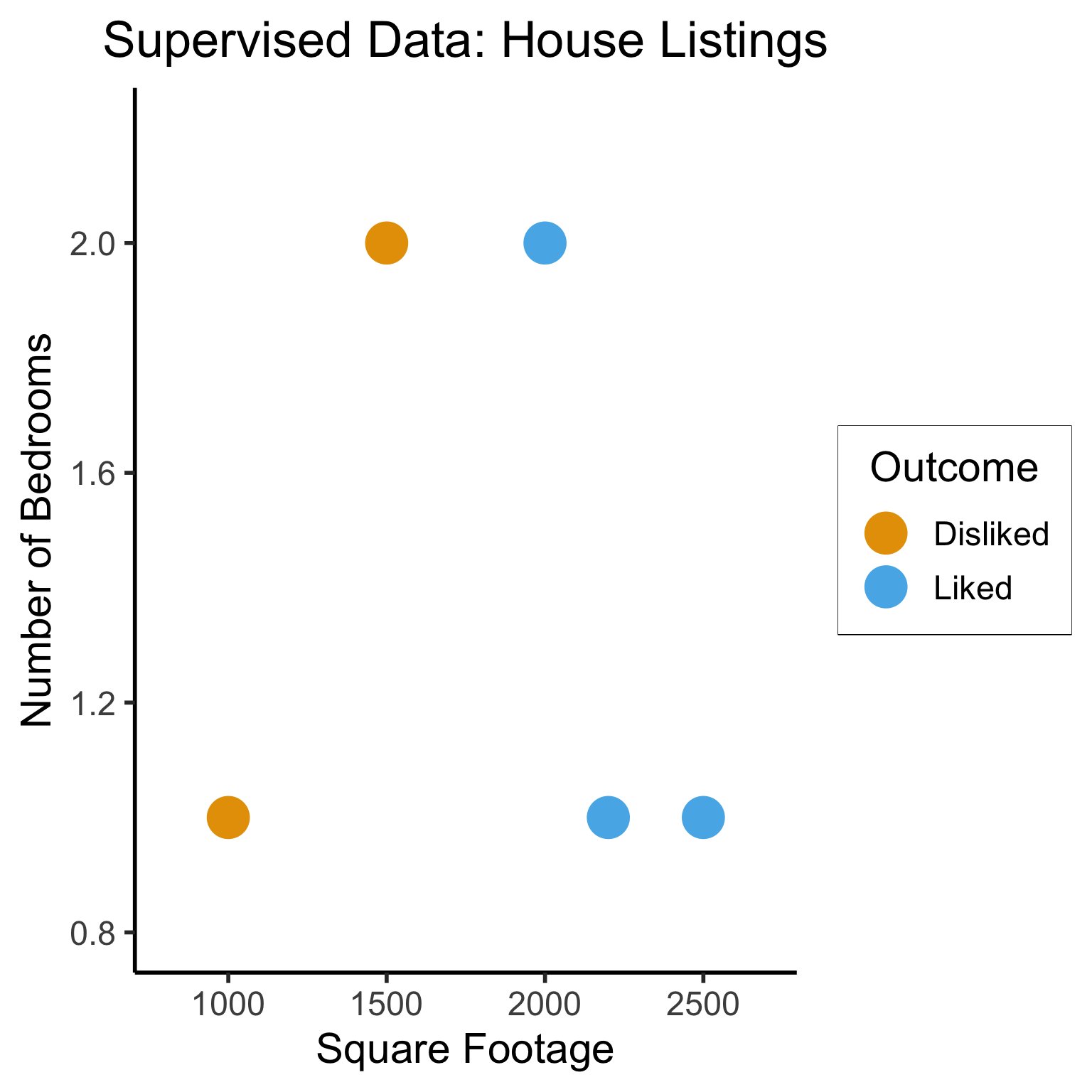

library(dplyr)

Attaching package: 'dplyr'

The following objects are masked from 'package:stats':

    filter, lag

The following objects are masked from 'package:base':

    intersect, setdiff, setequal, union

# To force a legend
unsup_grouped <- unsup_data |> mutate(big=bedrooms > 1)
unsup_grouped[['big']] <- factor(unsup_grouped[['big']], labels=c("?1","?2"))
ggplot(unsup_grouped, aes(x=sqft, y=bedrooms, fill=big)) + 
  geom_point(size = g_pointsize * 2) +
  labs(
    x = "Square Footage",
    y = "Number of Bedrooms",
    fill = "?"
  ) +
  dsan_theme("half") +
  expand_limits(x=c(800,2700), y=c(0.8,2.2)) +
  ggtitle("Unsupervised Data: House Listings") +
  theme(legend.background = element_rect(fill="white", color="white"), legend.box.background = element_rect(fill="white"), legend.text = element_text(color="white"), legend.title = element_text(color="white"), legend.position = "right") +
  scale_fill_discrete(labels=c("?","?")) +
  #scale_color_discrete(values=c("white","white"))
  scale_color_manual(name=NULL, values=c("white","white")) +
  #scale_color_manual(values=c("?1"="white","?2"="white"))
  guides(fill = guide_legend(override.aes = list(shape = NA)))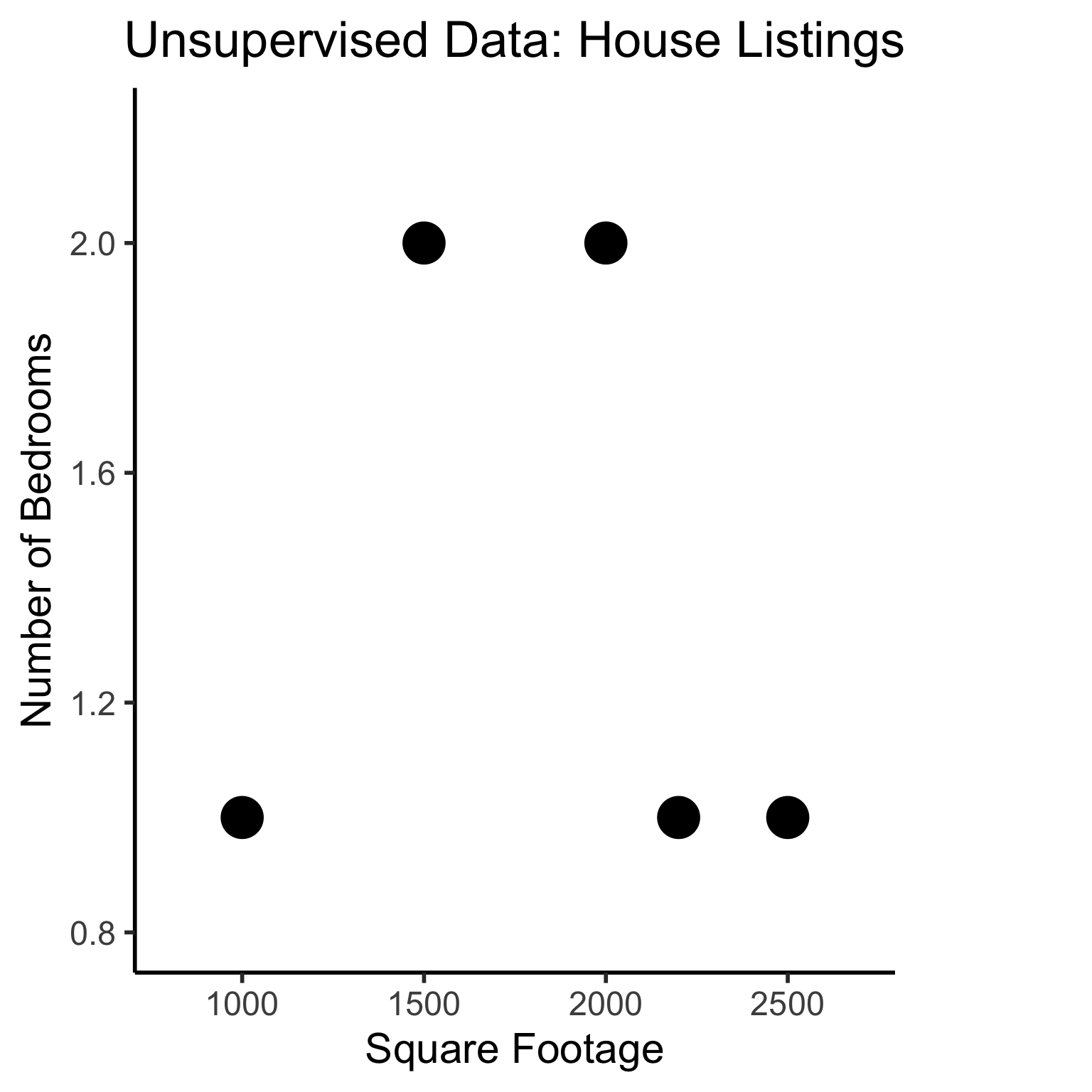

Different Goals

ggplot(sup_data, aes(x=sqft, y=bedrooms, color=rating)) + 
  geom_point(size = g_pointsize * 2) +
  labs(
    title = "Supervised Data: House Listings",
    x = "Square Footage",
    y = "Number of Bedrooms",
    color = "Outcome"
  ) +
  dsan_theme("half") +
  expand_limits(x=c(800,2700), y=c(0.8,2.2)) +
  geom_vline(xintercept = 1750, linetype="dashed", color = "black", size=1) +
  annotate('rect', xmin=-Inf, xmax=1750, ymin=-Inf, ymax=Inf, alpha=.2, fill=cbPalette[1]) +
  annotate('rect', xmin=1750, xmax=Inf, ymin=-Inf, ymax=Inf, alpha=.2, fill=cbPalette[2])

Warning: Using `size` aesthetic for lines was deprecated in ggplot2 3.4.0.
ℹ Please use `linewidth` instead.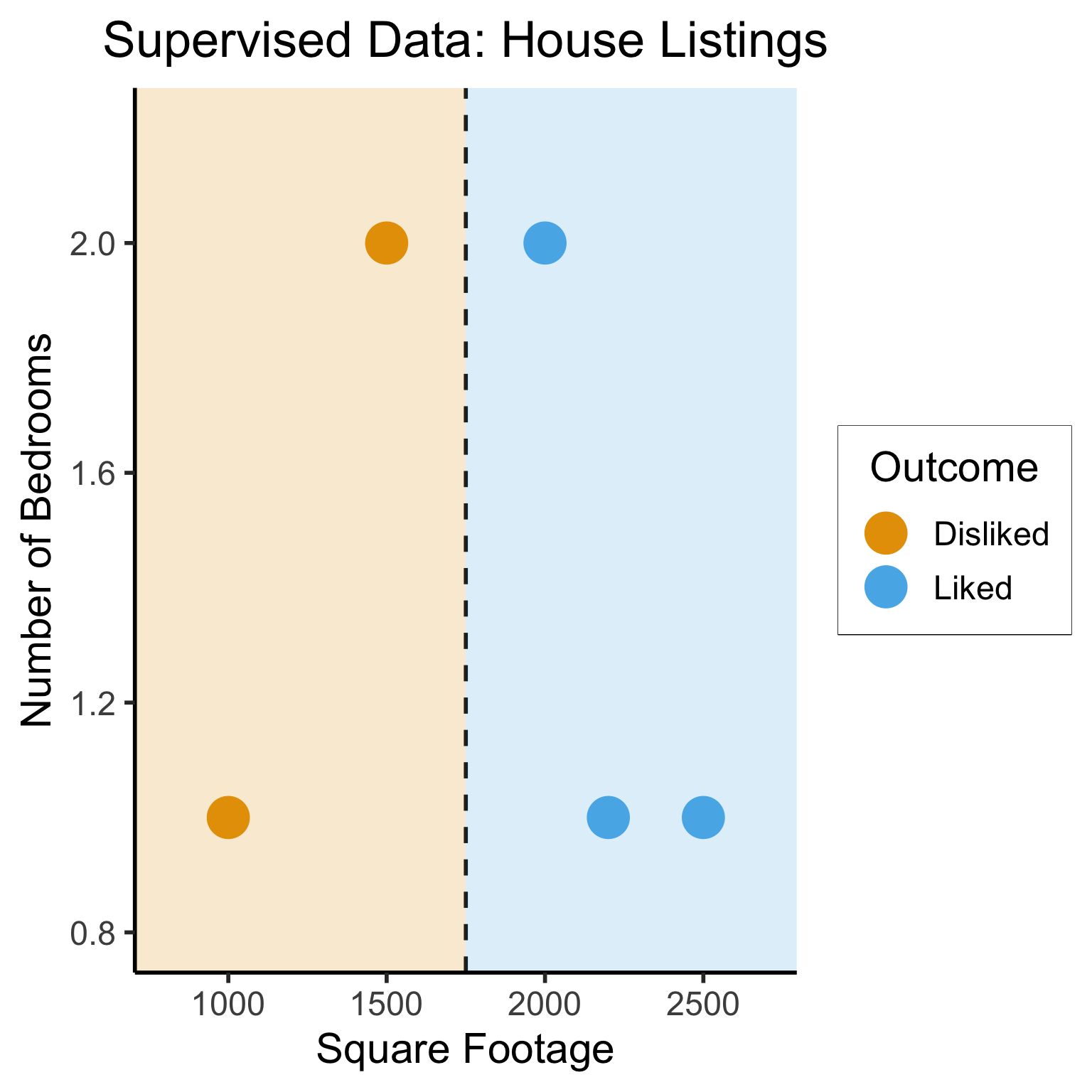

  #geom_rect(aes(xmin=-Inf, xmax=Inf, ymin=0, ymax=Inf, alpha=.2, fill='red'))

library(ggforce)
ggplot(unsup_grouped, aes(x=sqft, y=bedrooms)) +
  #scale_color_brewer(palette = "PuOr") +
  geom_mark_ellipse(expand=0.1, aes(fill=big), size = 1) +
  geom_point(size=g_pointsize * 2) +
  labs(
    x = "Square Footage",
    y = "Number of Bedrooms",
    fill = "?"
  ) +
  dsan_theme("half") +
  ggtitle("Unsupervised Data: House Listings") +
  #theme(legend.position = "none") +
  #theme(legend.title = text_element("?"))
  expand_limits(x=c(800,2700), y=c(0.8,2.2)) +
  scale_fill_manual(values=c(cbPalette[3],cbPalette[4]), labels=c("?","?"))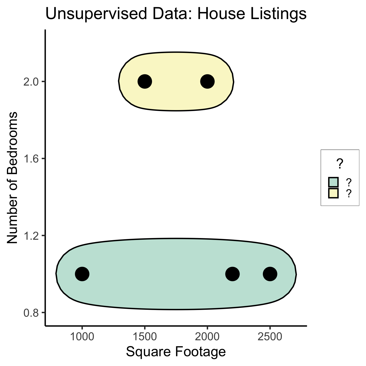

  #scale_fill_manual(labels=c("?","?"))

The “Learning” in Machine Learning

• Given these datasets, how do we learn the patterns?
• Naïve idea: Try random lines (each forming a decision boundary), pick “best” one

x_min <- 0
x_max <- 3000
y_min <- -1
y_max <- 3
rand_y0 <- runif(50, min=y_min, max=y_max)
rand_y1 <- runif(50, min=y_min, max=y_max)
rand_slope <- (rand_y1 - rand_y0)/(x_max - x_min)
rand_intercept <- rand_y0
rand_lines <- tibble::tibble(id=1:50, slope=rand_slope, intercept=rand_intercept)
#ggplot() +
#  geom_abline(data=rand_lines, aes(slope=slope, #intercept=intercept)) +
#  xlim(0,3000) +
#  ylim(0,2) +
#  dsan_theme()

ggplot(sup_data, aes(x=sqft, y=bedrooms, color=rating)) + 
  geom_point(size=g_pointsize) +
  labs(
    title = "The Like vs. Dislike Boundary: 50 Guesses",
    x = "Square Footage",
    y = "Number of Bedrooms",
    color = "Outcome"
  ) +
  dsan_theme() +
  expand_limits(x=c(800,2700), y=c(0.8,2.2)) +
  geom_abline(data=rand_lines, aes(slope=slope, intercept=intercept), linetype="dashed")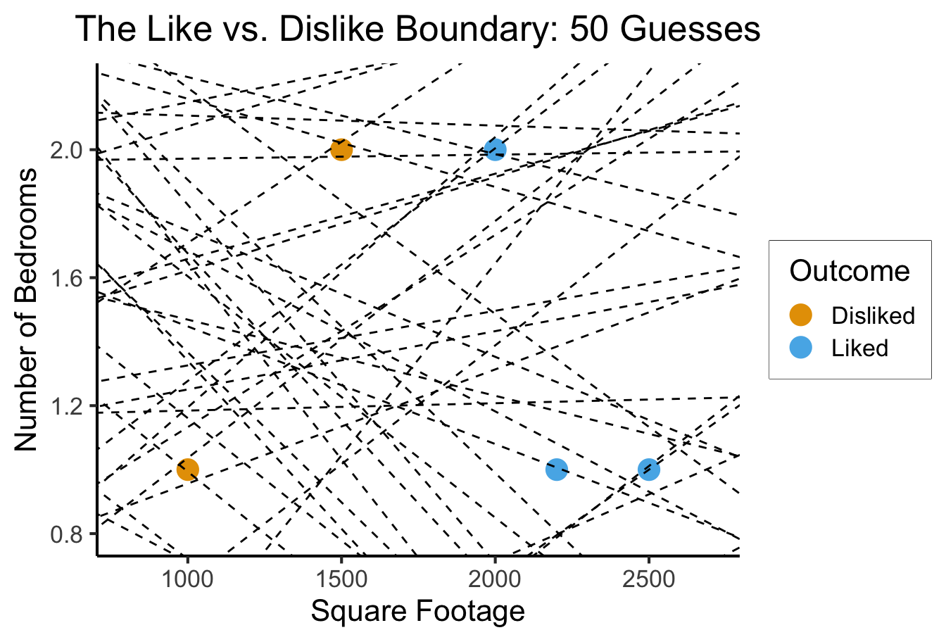

• What parameters are we choosing when we draw a random line? Random curve?

What Makes a “Good”/“Best” Guess?

• What’s your intuition? How about accuracy… 🤔

line_data <- tibble::tribble(
  ~id, ~slope, ~intercept,
  0, 0, 0.75,
  1, 0.00065, 0.5
)
data_range <- 800:2700
ribbon_range <- c(-Inf,data_range,Inf)
f1 <- function(x) { return(0*x + 0.75) }
f1_data <- tibble::tibble(line_x=ribbon_range,line_y=c(f1(700),f1(data_range),f1(3100)))
g1_plot <- ggplot(data=(line_data %>% filter(id==0))) +
  geom_abline(aes(slope=slope, intercept=intercept), linetype="dashed", size=1) +
  ggtitle("Guess 1: 60% Accuracy") +
  geom_point(data=sup_data, aes(x=sqft, y=bedrooms, color=rating), size=g_pointsize) +
  geom_ribbon(data=f1_data, aes(x=line_x, ymin=-Inf, ymax=line_y, fill="Disliked"), alpha=0.2) +
  geom_ribbon(data=f1_data, aes(x=line_x, ymin=line_y, ymax=Inf, fill="Liked"), alpha=0.2) +
  labs(
    x = "Square Footage",
    y = "Number of Bedrooms",
    color = "True Label"
  ) +
  dsan_theme() +
  expand_limits(x=data_range, y=c(0.8,2.2)) +
  scale_fill_manual(values=c("Liked"=cbPalette[2],"Disliked"=cbPalette[1]), name="Guess")

library(patchwork)
f2 <- function(x) { return(0.00065*x + 0.5) }
f2_data <- tibble::tibble(line_x=ribbon_range,line_y=c(f2(710),f2(data_range),f2(Inf)))
g2_plot <- ggplot(data=(line_data %>% filter(id==1))) +
  geom_abline(aes(slope=slope, intercept=intercept), linetype="dashed", size=1) +
  ggtitle("Guess 2: 60% Accuracy") +
  geom_point(data=sup_data, aes(x=sqft, y=bedrooms, color=rating), size=g_pointsize) +
  labs(
    x = "Square Footage",
    y = "Number of Bedrooms",
    color = "True Label"
  ) +
  geom_ribbon(data=f2_data, aes(x=line_x, ymin=-Inf, ymax=line_y, fill="Liked"), alpha=0.2) +
  geom_ribbon(data=f2_data, aes(x=line_x, ymin=line_y, ymax=Inf, fill="Disliked"), alpha=0.2) +
  dsan_theme() +
  expand_limits(x=data_range, y=c(0.8,2.2)) +
  scale_fill_manual(values=c("Liked"=cbPalette[2],"Disliked"=cbPalette[1]), name="Guess")

g1_plot + g2_plot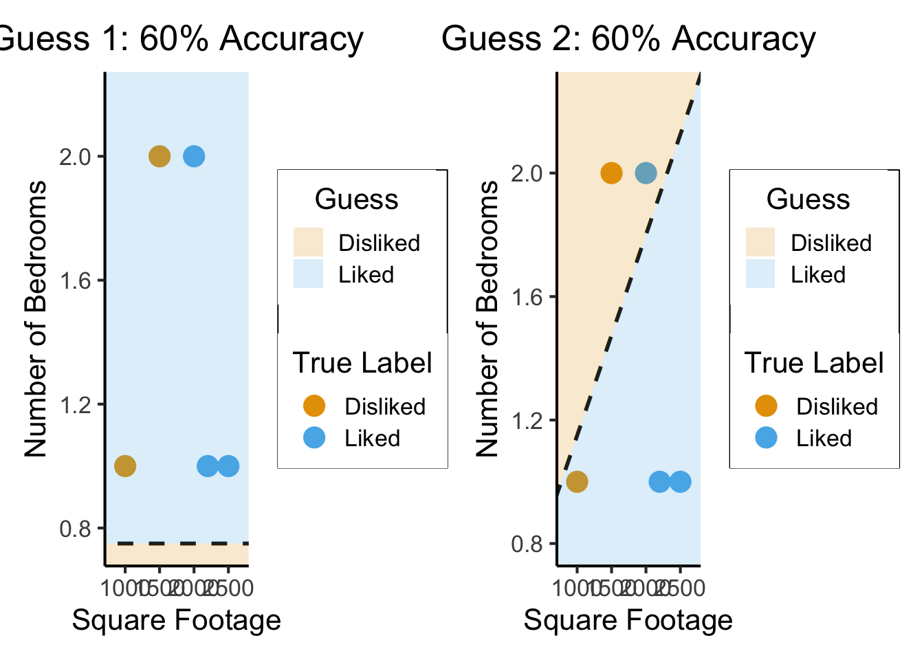

So… what’s wrong here?

What’s Wrong with Accuracy?

gen_homes <- function(n) {
  rand_sqft <- runif(n, min=2000, max=3000)
  rand_bedrooms <- sample(c(1,2), size=n, prob=c(0.5,0.5), replace=TRUE)
  rand_ids <- 1:n
  rand_rating <- "Liked"
  rand_tibble <- tibble::tibble(home_id=rand_ids, sqft=rand_sqft, bedrooms=rand_bedrooms, rating=rand_rating)
  return(rand_tibble)
}
fake_homes <- gen_homes(18)
fake_sup_data <- dplyr::bind_rows(sup_data, fake_homes)
line_data <- tibble::tribble(
  ~id, ~slope, ~intercept,
  0, 0, 0.75,
  1, 0.00065, 0.5
)
f1 <- function(x) { return(0*x + 0.75) }
f2 <- function(x) { return(0.00065*x + 0.5) }
# And check accuracy
fake_sup_data <- fake_sup_data %>% mutate(boundary1=f1(sqft)) %>% mutate(guessDislike1 = bedrooms < boundary1) %>% mutate(correct1 = ((rating=="Disliked") & (guessDislike1)) | (rating=="Liked") & (!guessDislike1))
fake_sup_data <- fake_sup_data %>% mutate(boundary2=f2(sqft)) %>% mutate(guessDislike2 = bedrooms > boundary2) %>% mutate(correct2 = ((rating=="Disliked") & (guessDislike2)) | (rating=="Liked") & (!guessDislike2))

data_range <- 800:2700
ribbon_range <- c(-Inf,data_range,Inf)

f1_data <- tibble::tibble(line_x=ribbon_range,line_y=c(f1(700),f1(data_range),f1(3200)))
g1_plot <- ggplot(data=(line_data %>% filter(id==0))) +
  geom_abline(aes(slope=slope, intercept=intercept), linetype="dashed", size=1) +
  ggtitle("Guess 1: 91.3% Accuracy") +
  geom_point(data=fake_sup_data, aes(x=sqft, y=bedrooms, fill=rating, color=rating, shape=factor(correct1, levels=c(TRUE,FALSE))), size=g_pointsize) +
  scale_shape_manual(values=c(24, 25)) +
  geom_ribbon(data=f1_data, aes(x=line_x, ymin=-Inf, ymax=line_y, fill="Disliked"), alpha=0.2) +
  geom_ribbon(data=f1_data, aes(x=line_x, ymin=line_y, ymax=Inf, fill="Liked"), alpha=0.2) +
  labs(
    x = "Square Footage",
    y = "Number of Bedrooms",
    color = "True Label",
    shape = "Correct Guess"
  ) +
  dsan_theme() +
  expand_limits(x=data_range, y=c(0.8,2.2)) +
  scale_fill_manual(values=c("Liked"=cbPalette[2],"Disliked"=cbPalette[1]), name="Guess")


f2_data <- tibble::tibble(line_x=ribbon_range,line_y=c(f2(700),f2(data_range),f2(3100)))
g2_plot <- ggplot(data=(line_data %>% filter(id==1))) +
  geom_abline(aes(slope=slope, intercept=intercept), linetype="dashed", size=1) +
  ggtitle("Guess 2: 73.9% Accuracy") +
  geom_point(data=fake_sup_data, aes(x=sqft, y=bedrooms, fill=rating, color=rating, shape=factor(correct2, levels=c(TRUE,FALSE))), size=g_pointsize) +
  scale_shape_manual(values=c(24, 25)) +
  labs(
    x = "Square Footage",
    y = "Number of Bedrooms",
    color = "True Label",
    shape = "Correct Guess"
  ) +
  geom_ribbon(data=f2_data, aes(x=line_x, ymin=-Inf, ymax=line_y, fill="Liked"), alpha=0.2) +
  geom_ribbon(data=f2_data, aes(x=line_x, ymin=line_y, ymax=Inf, fill="Disliked"), alpha=0.2) +
  dsan_theme() +
  expand_limits(x=data_range, y=c(0.8,2.2)) +
  scale_fill_manual(values=c("Liked"=cbPalette[2],"Disliked"=cbPalette[1]), name="Guess")

g1_plot + g2_plot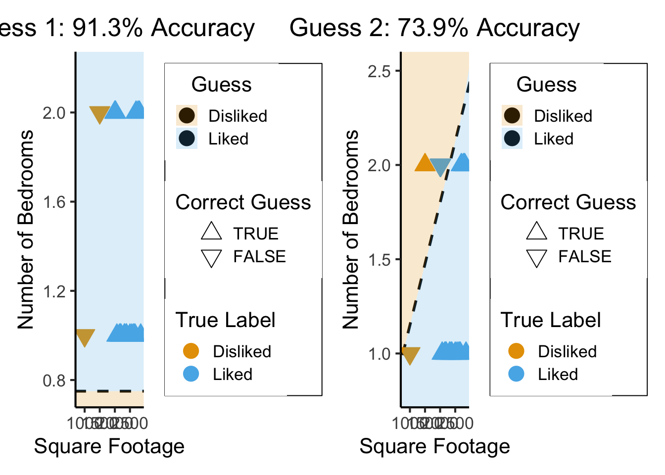

The (Oversimplified) Big Picture

• A model: some representation of something in the world

• How well does our model represent the world?² \(\mathsf{Correspondence}(y_{obs}, \theta)\)

• \(P\left(y_{obs}, \theta\right)\), \(P\left(\theta \; | \; y_{obs}\right)\), \(P\left(y_{obs} \; | \; \theta\right)\)³

• Maximum Likelihood Estimation?

\[ \begin{align*} \mathsf{Correspondence}(y_{obs}, \theta) &\equiv P(y = y_{obs}, \theta) \\ P(y = y_{obs}, \theta) &= P(y=y_{obs} \; | \; \theta)P(\theta) \\ &\propto P\left(y = y_{obs} \; | \; \theta\right)\ldots \implies \text{(maximize this!)} \\ \end{align*} \]

Measuring Errors: F1 Score

• How can we reward guesses which best discriminate between classes?

\[ \begin{align*} \mathsf{Precision} &= \frac{\# \text{true positives}}{\# \text{predicted positive}} = \frac{tp}{tp+fp} \\[1.5em] \mathsf{Recall} &= \frac{\# \text{true positives}}{\# \text{positives in data}} = \frac{tp}{tp+fn} \\[1.5em] F_1 &= 2\frac{\mathsf{Precision} \cdot \mathsf{Recall}}{\mathsf{Precision} + \mathsf{Recall}} = \mathsf{HMean}(\mathsf{Precision}, \mathsf{Recall}) \end{align*} \]

• Think about: How does this address/fix issue with accuracy?

Here \(\mathsf{HMean}\) is the Harmonic Mean function: see appendix slide or Wikipedia.

Measuring Errors: The Loss Function

• What about regression?
  • No longer just “true prediction good, false prediction bad”
• We have to quantify how bad the guess is! Then we can scale the penalty accordingly: \(\text{penalty} \propto \text{badness}\)
• Enter Loss Functions! Just distances (using distance metrics you’ve already seen) between the true value and our guess:
  • Squared Error \(L^2(y_{obs}, y_{pred}) = (y_{obs} - y_{pred})^2\)
  • Kullback-Leibler Divergence if guessing distributions

Calculus Rears its Ugly Head

• Neural networks use derivatives/gradients to improve their predictions given a particular loss function.

base <-
  ggplot() +
  xlim(-5, 5) +
  ylim(0, 25) +
  labs(
    x = "Y[obs] - Y[pred]",
    y = "Prediction Badness (Loss)"
  ) +
  dsan_theme()

my_fn <- function(x) { return(x^2) }
my_deriv2 <- function(x) { return(4*x - 4) }
my_derivN4 <- function(x) { return(-8*x - 16) }
base + geom_function(fun = my_fn, color=cbPalette[1], linewidth=1) +
  geom_point(data=as.data.frame(list(x=2,y=4)), aes(x=x,y=y), color=cbPalette[2], size=g_pointsize/2) + 
  geom_function(fun = my_deriv2, color=cbPalette[2], linewidth=1) +
  geom_point(data=as.data.frame(list(x=-4,y=16)), aes(x=x,y=y), color=cbPalette[3], size=g_pointsize/2) + 
  geom_function(fun = my_derivN4, color=cbPalette[3], linewidth=1)

Warning: Removed 60 rows containing missing values or values outside the scale range
(`geom_function()`).

Warning: Removed 70 rows containing missing values or values outside the scale range
(`geom_function()`).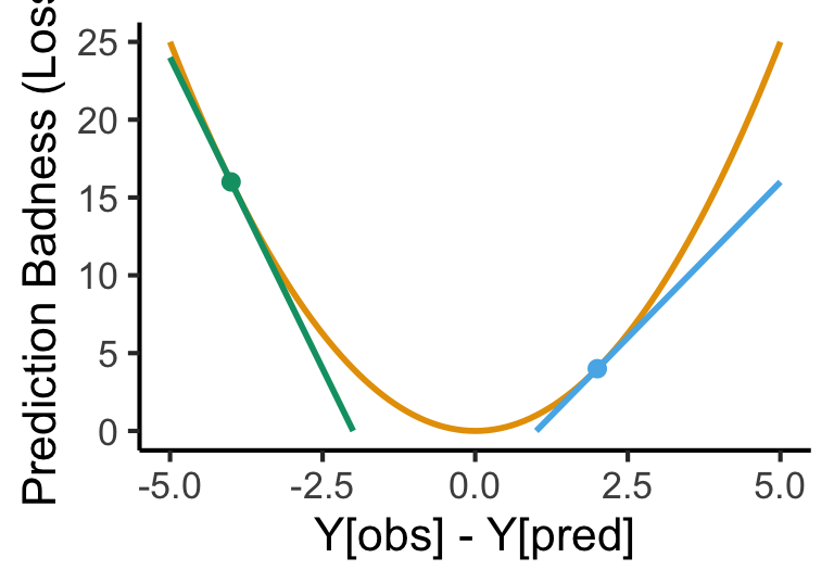

my_fake_deriv <- function(x) { return(-x) }
my_fake_deriv2 <- function(x) { return(-(1/2)*x + 1/2) }
my_fake_deriv3 <- function(x) { return(-(1/4)*x + 3/4) }

d=data.frame(x=c(-2,-1,0,1,2), y=c(1,0,0,1,1))
base <- ggplot() +
  xlim(-5,5) +
  ylim(0,2) +
  labs(
    x="Y[obs] - Y[pred]",
    y="Prediction Badness (Loss)"
  ) +
  geom_step(data=d, mapping=aes(x=x, y=y), linewidth=1) +
  dsan_theme()

base + geom_point(data=as.data.frame(list(x=2,y=4)), aes(x=x,y=y), color=cbPalette[2], size=g_pointsize/2) + 
  geom_function(fun = my_fake_deriv, color=cbPalette[2], linewidth=1) +
  geom_function(fun = my_fake_deriv2, color=cbPalette[3], linewidth=1) +
  geom_function(fun = my_fake_deriv3, color=cbPalette[4], linewidth=1) +
  geom_point(data=as.data.frame(list(x=-1,y=1)), aes(x=x,y=y), color=cbPalette[2], size=g_pointsize/2) +
  annotate("text", x = -0.7, y = 1.1, label = "?", size=6)

Warning: Removed 1 row containing missing values or values outside the scale range
(`geom_point()`).

Warning: Removed 80 rows containing missing values or values outside the scale range
(`geom_function()`).

Warning: Removed 60 rows containing missing values or values outside the scale range
(`geom_function()`).

Warning: Removed 20 rows containing missing values or values outside the scale range
(`geom_function()`).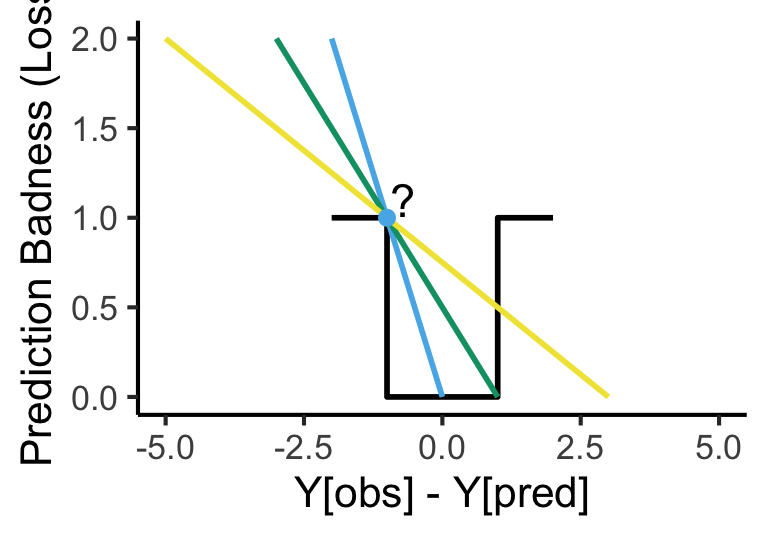

• Can we just use the \(F_1\) score?

\[ \frac{\partial F_1(weights)}{\partial weights} = \ldots \; ? \; \ldots 💀 \]

Quantifying Discrete Loss

• We can quantify a differentiable discrete loss by asking the algorithm how confident it is
  • Closer to 0 \(\implies\) more confident that the true label is 0
  • Closer to 1 \(\implies\) more confident that the true label is 1

\[ \mathcal{L}_{CE}(y_{pred}, y_{obs}) = -(y_{obs}\log(y_{pred}) + (1-y_{obs})\log(1-y_{pred})) \]

y_pred <- seq(from = 0, to = 1, by = 0.001)
compute_ce <- function(y_p, y_o) { return(-(y_o * log(y_p) + (1-y_o)*log(1-y_p))) }
ce0 <- compute_ce(y_pred, 0)
ce1 <- compute_ce(y_pred, 1)
ce0_data <- tibble::tibble(y_pred=y_pred, y_obs=0, ce=ce0)
ce1_data <- tibble::tibble(y_pred=y_pred, y_obs=1, ce=ce1)
ce_data <- dplyr::bind_rows(ce0_data, ce1_data)
ggplot(ce_data, aes(x=y_pred, y=ce, color=factor(y_obs))) +
  geom_line(linewidth=1) +
  labs(
    title="Binary Cross-Entropy Loss",
    x = "Predicted Value",
    y = "Loss",
    color = "Actual Value"
  ) +
  dsan_theme() +
  ylim(0,6)

Warning: Removed 2 rows containing missing values or values outside the scale range
(`geom_line()`).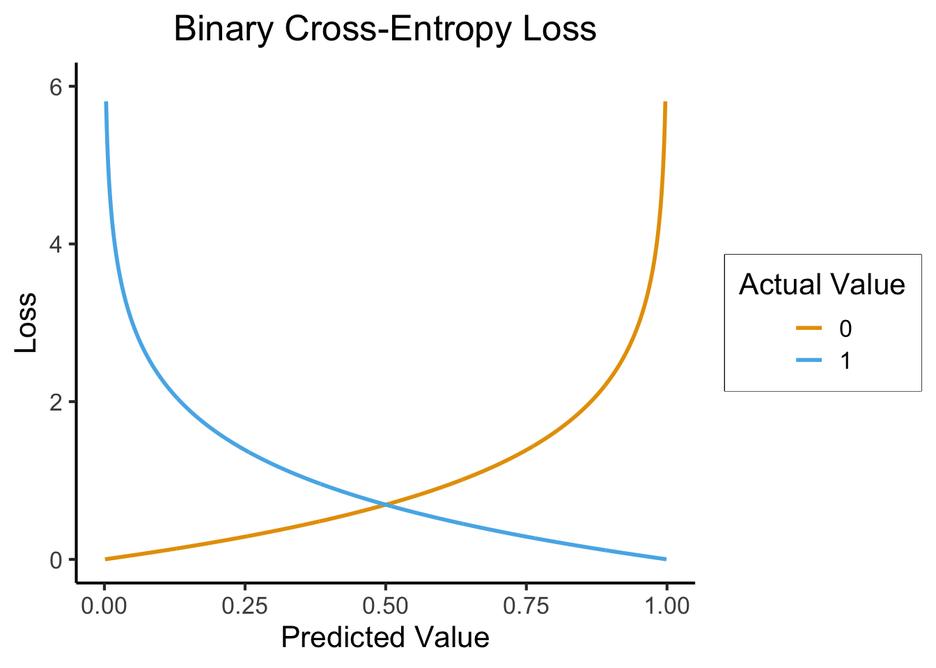

Loss Function \(\implies\) Ready to Learn!

• Once we’ve chosen a loss function, the learning algorithm has what it needs to proceed with the actual learning

• Notation: Bundle all the model’s parameters together into \(\theta\)

• The goal: \[ \min_{\theta} \mathcal{L}(y_{obs}, y_{pred}(\theta)) \]

• What would this look like for the random-lines approach?

• Is there a more efficient way?

Calculus Strikes Again

• tldr: The slope of a function tells us how to get to a minimum (why a minimum rather than the minimum?)
• Derivative (gradient) = “direction of sharpest decrease”
• Think of hill climbing! Let \(\ell_t \in L\) be your location at time \(t\), and \(Alt(\ell)\) be the altitude at a location \(\ell\)
• Gradient descent for \(\ell^* = \max_{\ell \in L} Alt(\ell)\): \[ \ell_{t+1} = \ell_t + \gamma\nabla Alt(\ell_t),\ t\geq 0. \]
• While top of mountain = good, Loss is bad: we want to find the bottom of the “loss crater”
  • \(\implies\) we do the opposite: subtract \(\gamma\nabla Alt(\ell_t)\)

Good and Bad News

• Universal Approximation Theorem
• Neural networks can represent any function mapping one Euclidean space to another
• (Neural Turing Machines:)

Figure from @schmidinger_exploring_2019

• Weierstrass Approximation Theorem
• (Polynomials could already represent any function)

\[ f \in C([a,b],[a,b]) \] \[ \implies \forall \epsilon > 0, \exists p \in \mathbb{R}[x] : \] \[ \forall x \in [a, b] \; \left|f(x) − p(x)\right| < \epsilon \]

• Implications for machine learning?

So What’s the Issue?

x <- seq(from = 0, to = 1, by = 0.1)
n <- length(x)
eps <- rnorm(n, 0, 0.04)
y <- x + eps
# But make one big outlier
midpoint <- ceiling((3/4)*n)
y[midpoint] <- 0
of_data <- tibble::tibble(x=x, y=y)
# Linear model
lin_model <- lm(y ~ x)
# But now polynomial regression
poly_model <- lm(y ~ poly(x, degree = 10, raw=TRUE))
#summary(model)

ggplot(of_data, aes(x=x, y=y)) +
  geom_point(size=g_pointsize/2) +
  labs(
    title = "Training Data",
    color = "Model"
  ) +
  dsan_theme()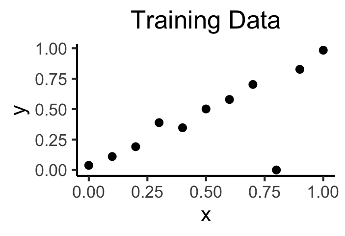

ggplot(of_data, aes(x=x, y=y)) +
  geom_point(size=g_pointsize/2) +
  geom_abline(aes(intercept=0, slope=1, color="Linear"), linewidth=1, show.legend = FALSE) +
  stat_smooth(method = "lm",
              formula = y ~ poly(x, 10, raw=TRUE),
              se = FALSE, aes(color="Polynomial")) +
  labs(
    title = "A Perfect Model?",
    color = "Model"
  ) +
  dsan_theme()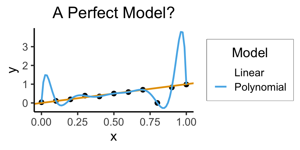

• Higher \(R^2\) = Better Model? Lower \(RSS\)?
• Linear Model:

summary(lin_model)$r.squared

[1] 0.5269359

get_rss(lin_model)

[1] 0.5075188

• Polynomial Model:

summary(poly_model)$r.squared

[1] 1

get_rss(poly_model)

[1] 0

Generalization

• Training Accuracy: How well does it fit the data we can see?
• Test Accuracy: How well does it generalize to future data?

# Data setup
x_test <- seq(from = 0, to = 1, by = 0.1)
n_test <- length(x_test)
eps_test <- rnorm(n_test, 0, 0.04)
y_test <- x_test + eps_test
of_data_test <- tibble::tibble(x=x_test, y=y_test)
lin_y_pred_test <- predict(lin_model, as.data.frame(x_test))
#lin_y_pred_test
lin_resids_test <- y_test - lin_y_pred_test
#lin_resids_test
lin_rss_test <- sum(lin_resids_test^2)
#lin_rss_test
# Lin R2 = 1 - RSS/TSS
tss_test <- sum((y_test - mean(y_test))^2)
lin_r2_test <- 1 - (lin_rss_test / tss_test)
#lin_r2_test
# Now the poly model
poly_y_pred_test <- predict(poly_model, as.data.frame(x_test))
poly_resids_test <- y_test - poly_y_pred_test
poly_rss_test <- sum(poly_resids_test^2)
#poly_rss_test
# RSS
poly_r2_test <- 1 - (poly_rss_test / tss_test)
#poly_r2_test

ggplot(of_data, aes(x=x, y=y)) +
  stat_smooth(method = "lm",
              formula = y ~ poly(x, 10, raw = TRUE),
              se = FALSE, aes(color="Polynomial")) +
  dsan_theme() +
  geom_point(data=of_data_test, aes(x=x_test, y=y_test), size=g_pointsize/2) +
  geom_abline(aes(intercept=0, slope=1, color="Linear"), linewidth=1, show.legend = FALSE) +
  labs(
    title = "Performance on Unseen Test Data",
    color = "Model"
  ) +
  dsan_theme()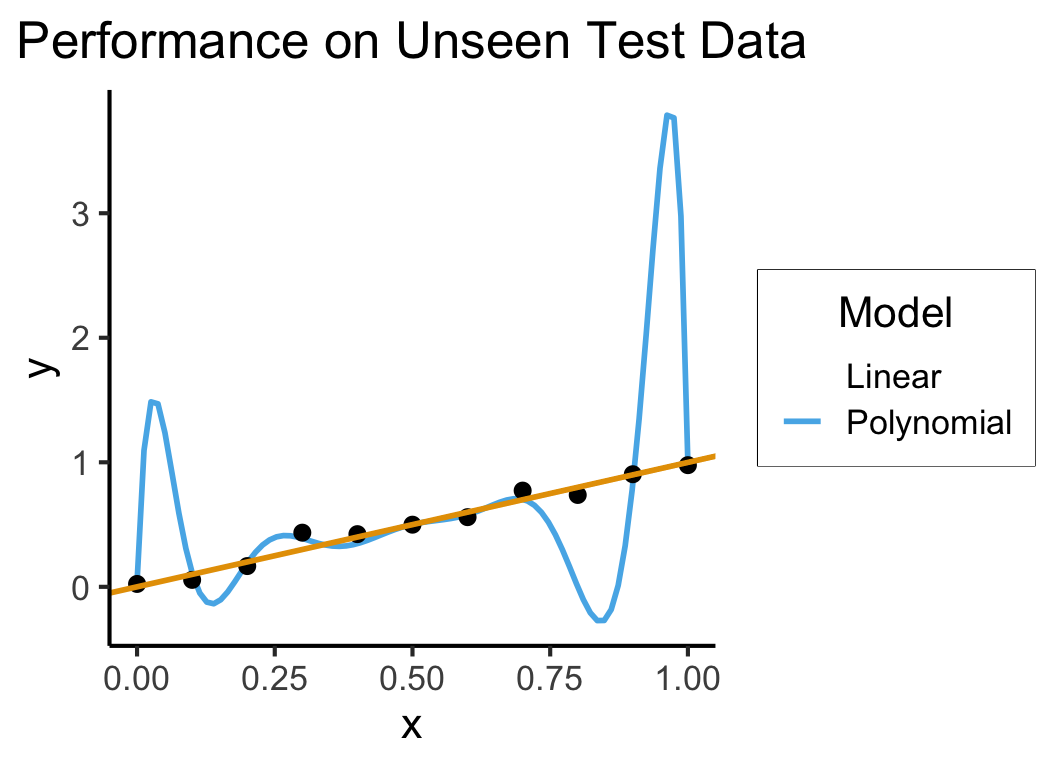

• Linear Model:

lin_r2_test

[1] 0.8366753

lin_rss_test

[1] 0.1749389

• Polynomial Model:

poly_r2_test

[1] 0.470513

poly_rss_test

[1] 0.5671394

How to Avoid Overfitting?

• The gist: penalize model complexity

Original optimization: \[ \theta^* = \underset{\theta}{\operatorname{argmin}} \mathcal{L}(y_{obs}, y_{pred}(\theta)) \]

New optimization: \[ \theta^* = \underset{\theta}{\operatorname{argmin}} \left[ \mathcal{L}(y_{obs}, y_{pred}(\theta)) + \mathsf{Complexity}(\theta) \right] \]

• So how do we measure, and penalize, “complexity”?

Regularization: Measuring and Penalizing Complexity

• In the case of polynomials, fairly simple complexity measure: degree of polynomial

\[ \mathsf{Complexity}(y_{pred} = \beta_0 + \beta_1 x + \beta_2 x^2 + \beta_3 x^3) > \mathsf{Complexity}(y_{pred} = \beta_0 + \beta_1 x) \]

• In general machine learning, however, we might not be working with polynomials
• In neural networks, for example, we sometimes toss in millions of features and ask the algorithm to “just figure it out”
• The gist, in the general case, is thus: try to “amplify” the most important features and shrink the rest, so that

\[ \mathsf{Complexity} \propto \frac{|\text{AmplifiedFeatures}|}{|\text{ShrunkFeatures}|} \]

LASSO and Elastic Net Regularization

• Many ways to translate this intuition into math!
• In several fields, however (econ, biostatistics), LASSO⁴ [@tibshirani_regression_1996] is standard:

\[ \beta^*_{LASSO} = {\underset{\beta}{\operatorname{argmin}}}\left\{{\frac {1}{N}}\left\|y-X\beta \right\|_{2}^{2}+\lambda \|\beta \|_{1}\right\} \]

• Why does this work to penalize complexity? What does the parameter \(\lambda\) do?
• Some known issues with LASSO fixed in extension of the same intuitions: Elastic Net

\[ \beta^*_{EN} = {\underset {\beta }{\operatorname {argmin} }}\left\{ \|y-X\beta \|^{2}_2+\lambda _{2}\|\beta \|^{2}+\lambda _{1}\|\beta \|_{1} \right\} \]

• (Ensures a unique global minimum! Note that \(\lambda_2 = 0, \lambda_1 = 1 \implies \beta^*_{LASSO} = \beta^*_{EN}\))

Training vs. Test Data

Cross-Validation

• The idea that good models generalize well is crucial!
  • What if we could leverage this insight to optimize over our training data?
  • The key: Validation Sets

Hyperparameters

• The unspoken (but highly consequential!) “settings” for our learning procedure (that we haven’t optimized via gradient descent)
• There are several we’ve already seen – can you name them?

• Unsupervised Clustering: The number of clusters we want (\(K\))
• Gradient Descent: The step size \(\gamma\)
• LASSO/Elastic Net: \(\lambda\)
• The train/validation/test split!

Hyperparameter Selection

• Every model comes with its own hyperparameters:
  • Neural Networks: Number of layers, number of nodes per layer
  • Decision Trees: Maximum tree depth, max number of features to include
  • Topic Models: Number of topics, document/topic priors
• So, how do we choose?
  • Often more art than science
  • Principled, universally applicable, but slow: grid search
  • Specific methods for specific algorithms: ADAM [@kingma_adam_2017] for Neural Network learning rates)

Appendix: Harmonic Mean

• \(\mathsf{HMean}\) is the harmonic mean, an alternative to the standard (arithmetic) mean
• Penalizes greater “gaps” between precision and recall: if precision is 0 and recall is 1, for example, their arithmetic mean is 0.5 while their harmonic mean is 0.
• For the curious: given numbers \(X = \{x_1, \ldots, x_n\}\), \(\mathsf{HMean}(X) = \frac{n}{\sum_{i=1}^nx_i^{-1}}\)

Footnotes

1. Whether standard classification (sorting observations into bins) or regression (assigning a real number to each observation)

2. Computer scientists implicitly assume a Correspondence Theory of Truth, hence the choice of name

3. Thanks to Bayes’ Rule, mathematically we can always convert between the two: \(P(A|B) = \frac{P(B|A)P(A)}{P(B)}\)

4. Least Absolute Shrinkage and Selection Operator