Extra Slides: A Slightly Deeper Dive Into Machine Learning

DSAN5000: Data Science and Analytics
(Addendum to Week 07)

Jeff Jacobs

jj1088@georgetown.edu

2025-01-22

Supervised vs. Unsupervised Learning

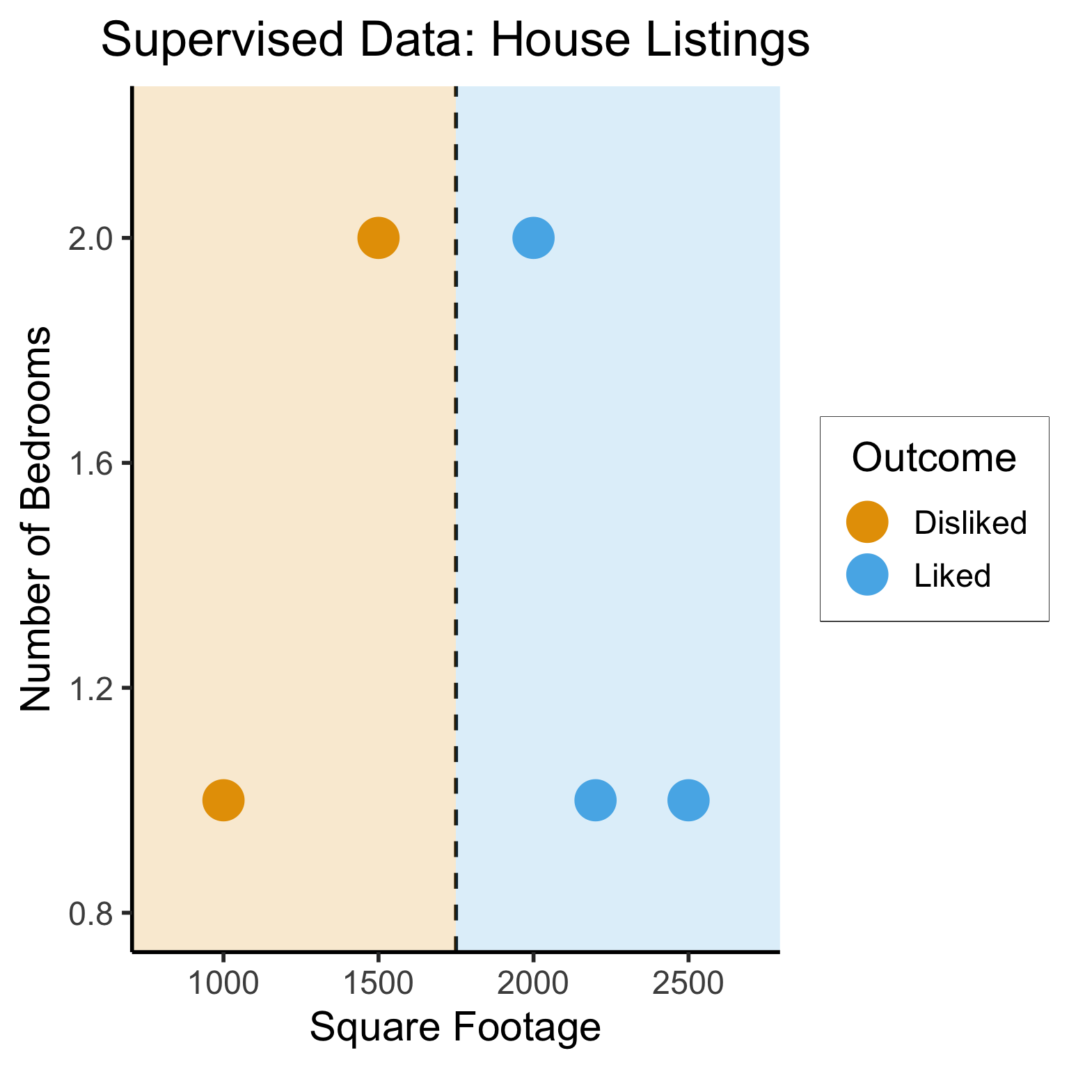
Supervised Learning: You want the computer to learn the existing pattern of how you are classifying¹ observations

• Discovering the relationship between properties of data and outcomes
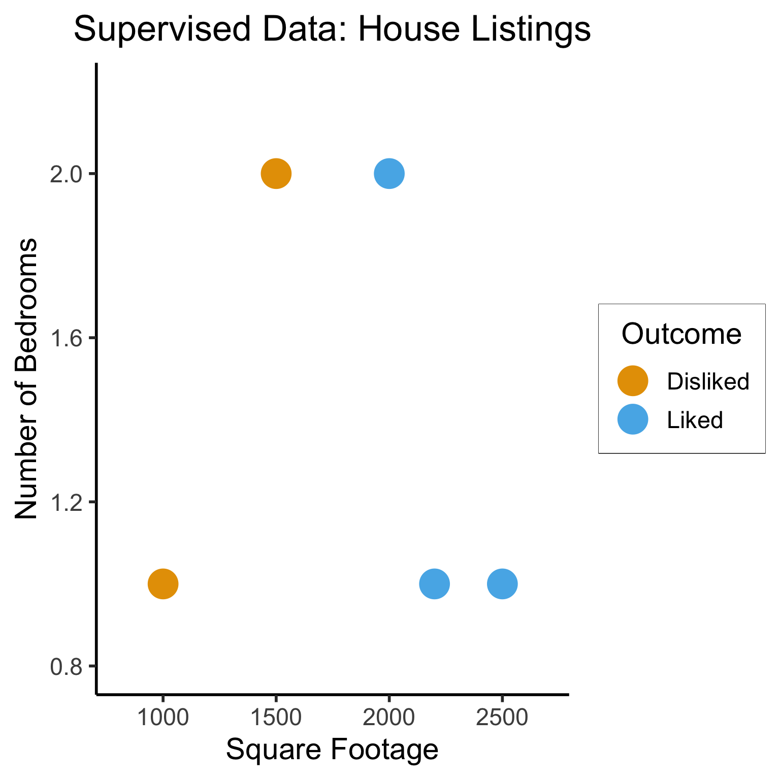
• Example (Binary Classification): I look at homes on Zillow, saving those I like to folder A and don’t like to folder B
• Example (Regression): I assign a rating of 0-100 to each home
• In both cases: I ask the computer to learn my schema (how I classify)

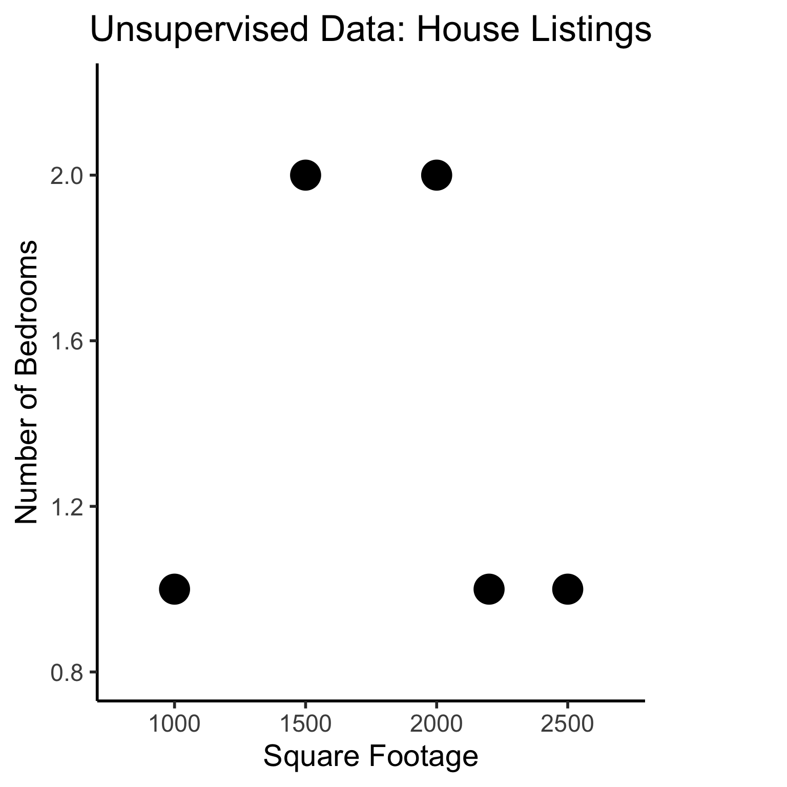
Unsupervised Learning: You want the computer to find patterns in a dataset, without any prior classification info

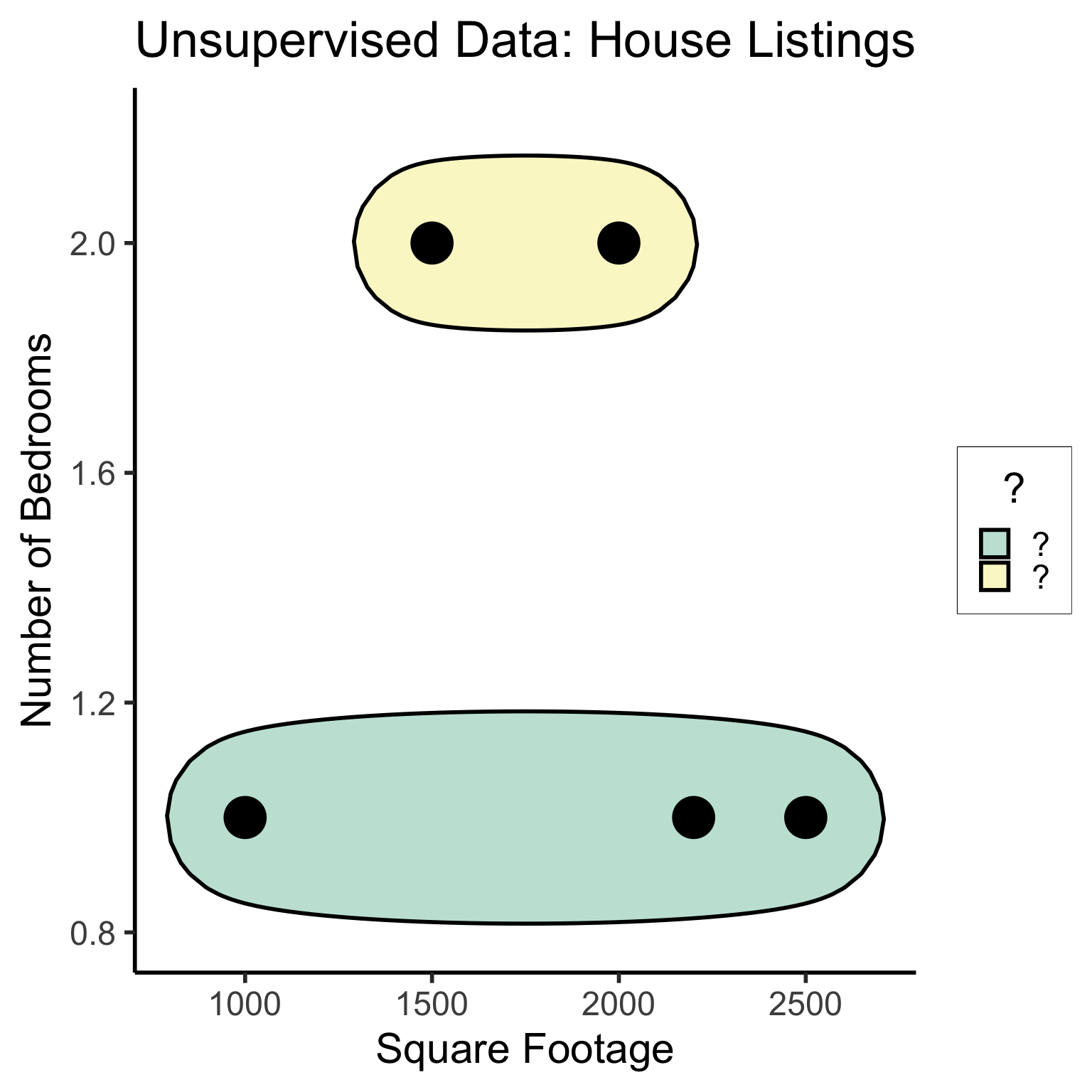
• Typically: grouping or clustering observations based on shared properties
• Example (Clustering): I save all the used car listings I can find, and ask the computer to “find a pattern” in this data, by clustering similar cars together

1. Whether standard classification (sorting observations into bins) or regression (assigning a real number to each observation)

Dataset Structures

Supervised Learning: Dataset has both explanatory variables (“features”) and response variables (“labels”)

home_id	sqft	bedrooms	rating
0	1000	1	Disliked
1	2000	2	Liked
2	2500	1	Liked
3	1500	2	Disliked
4	2200	1	Liked

Unsupervised Learning: Dataset has only explanatory variables (“features”)

home_id	sqft	bedrooms
0	1000	1
1	2000	2
2	2500	1
3	1500	2
4	2200	1

Dataset Structures: Visualized

Different Goals

The “Learning” in Machine Learning

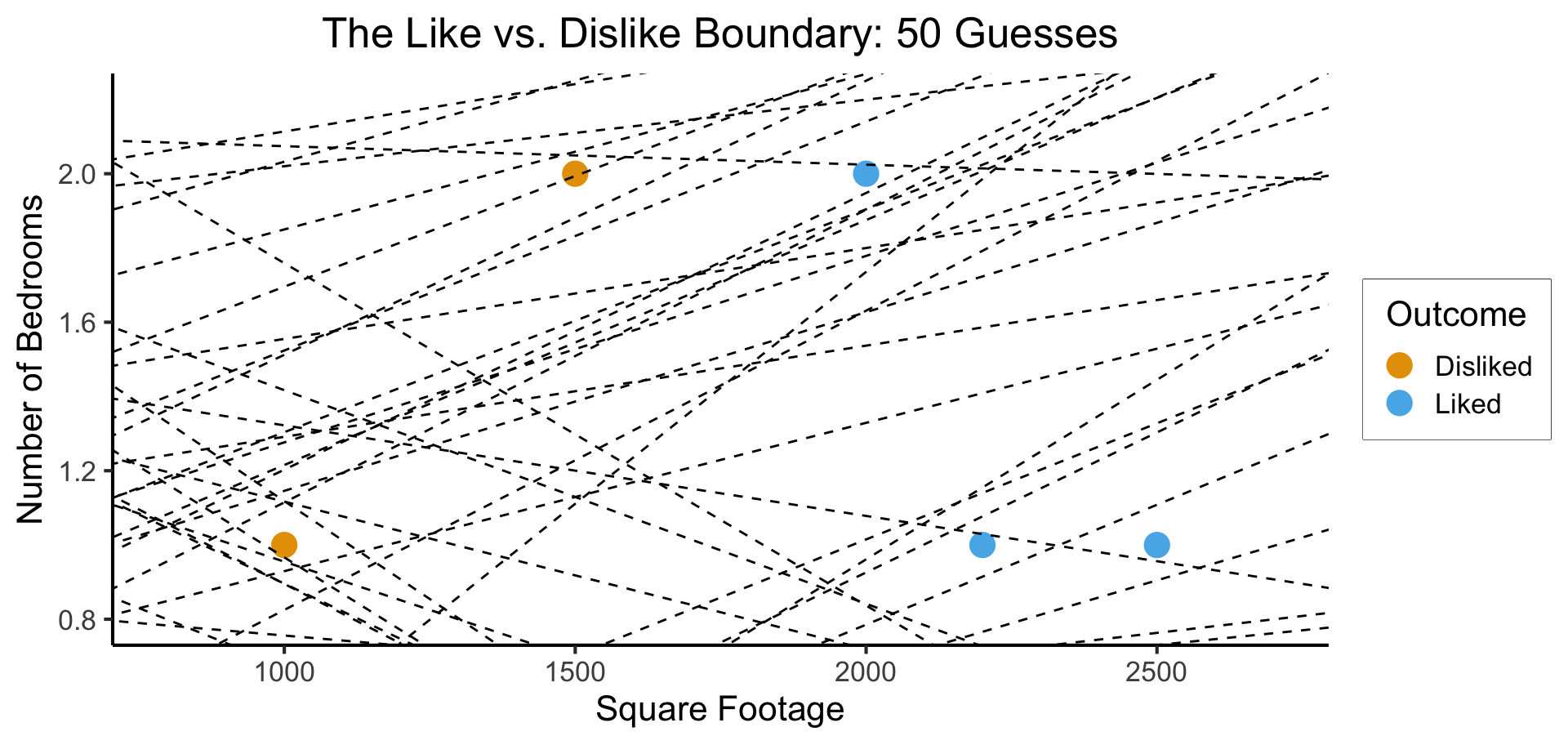
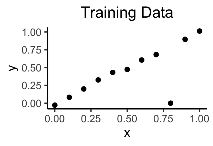
• Given these datasets, how do we learn the patterns?
• Naïve idea: Try random lines (each forming a decision boundary), pick “best” one

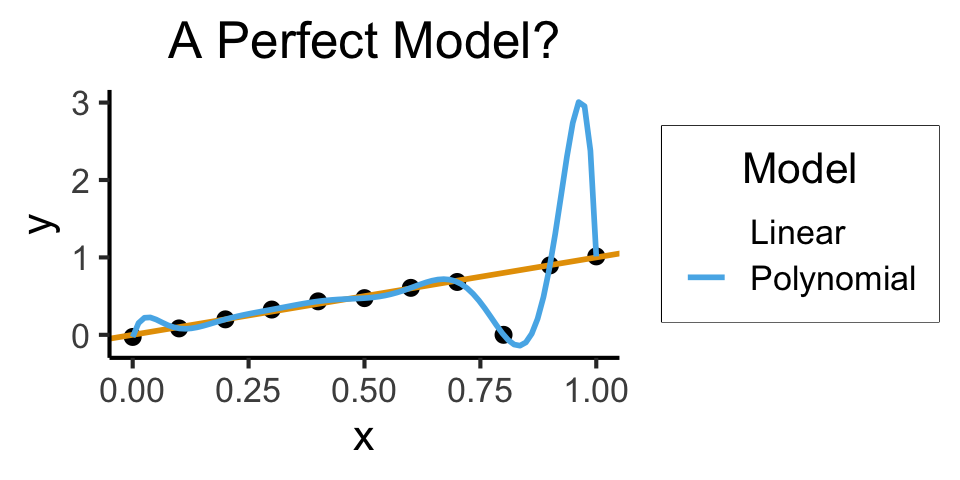
• What parameters are we choosing when we draw a random line? Random curve?

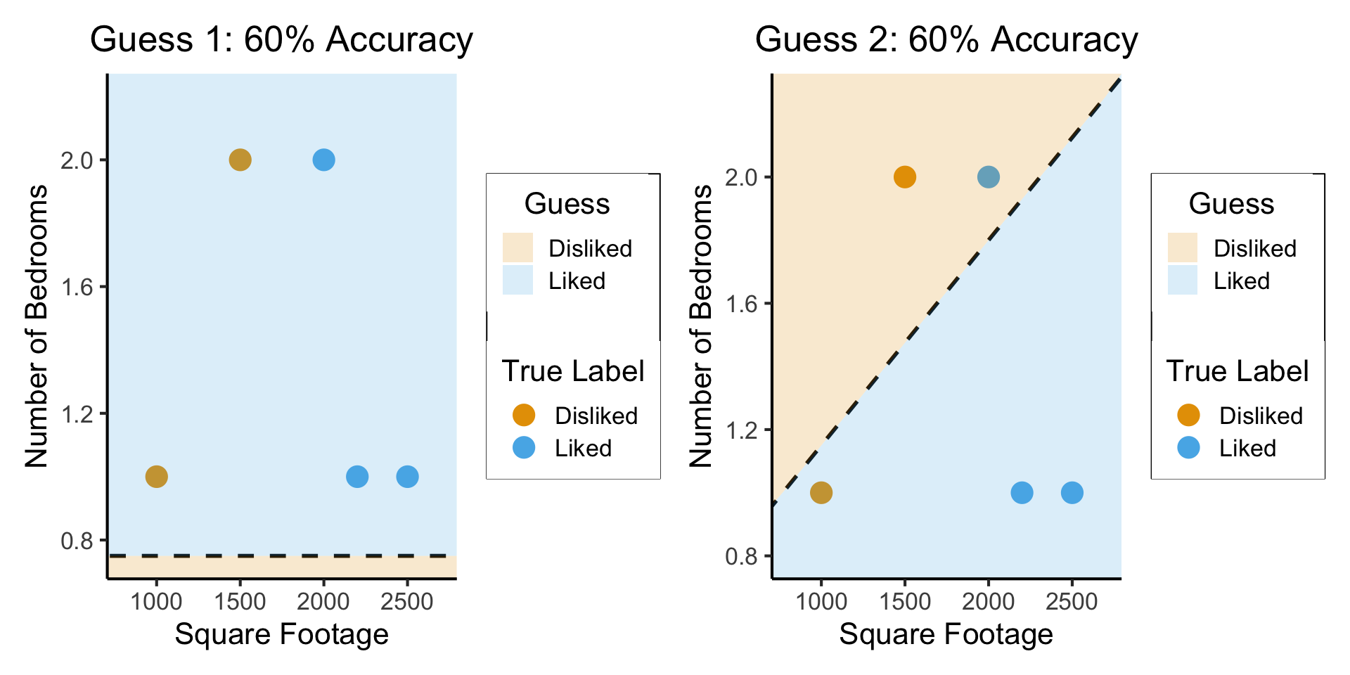
What Makes a “Good”/“Best” Guess?

• What’s your intuition? How about accuracy… 🤔

So… what’s wrong here?

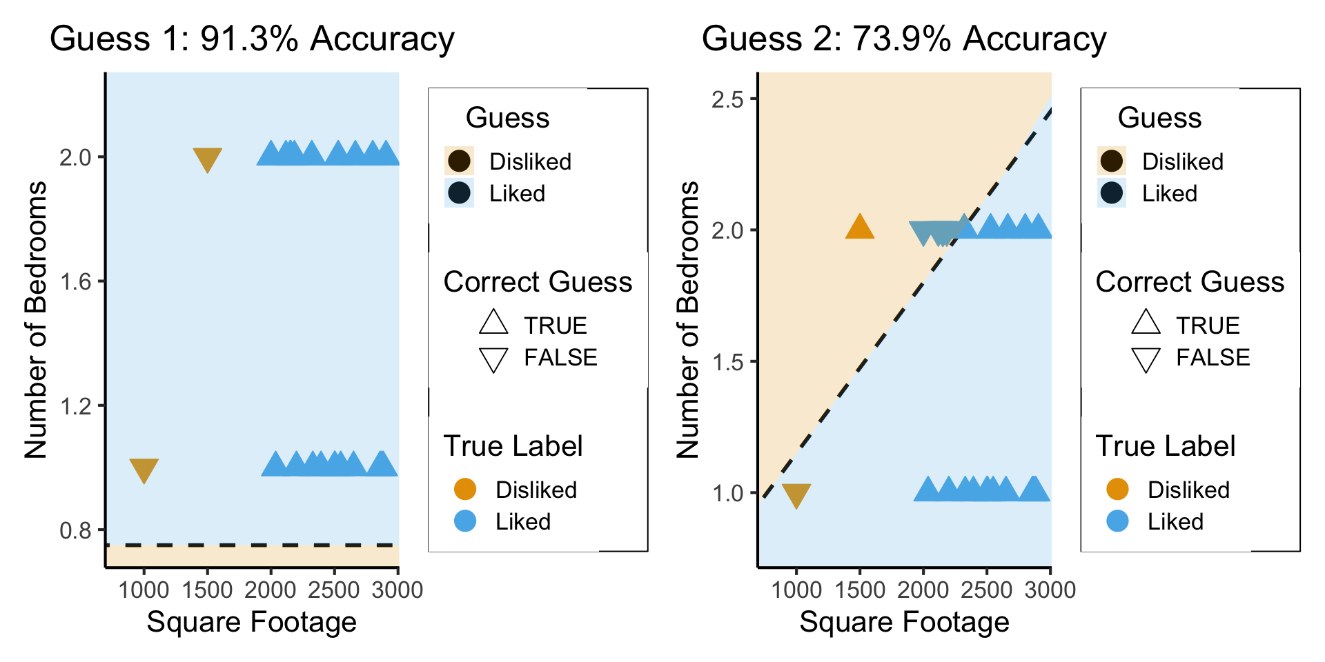
What’s Wrong with Accuracy?

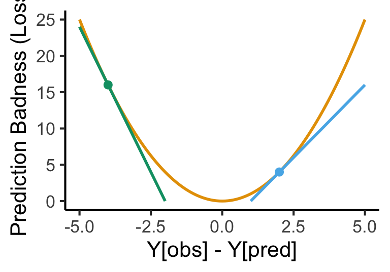
The (Oversimplified) Big Picture

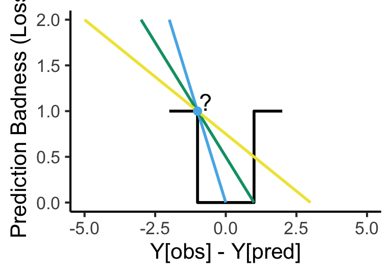
• A model: some representation of something in the world

• How well does our model represent the world?¹ \(\mathsf{Correspondence}(y_{obs}, \theta)\)

• \(P\left(y_{obs}, \theta\right)\), \(P\left(\theta \; | \; y_{obs}\right)\), \(P\left(y_{obs} \; | \; \theta\right)\)²

• Maximum Likelihood Estimation?

\[ \begin{align*} \mathsf{Correspondence}(y_{obs}, \theta) &\equiv P(y = y_{obs}, \theta) \\ P(y = y_{obs}, \theta) &= P(y=y_{obs} \; | \; \theta)P(\theta) \\ &\propto P\left(y = y_{obs} \; | \; \theta\right)\ldots \implies \text{(maximize this!)} \\ \end{align*} \]

1. Computer scientists implicitly assume a Correspondence Theory of Truth, hence the choice of name

2. Thanks to Bayes’ Rule, mathematically we can always convert between the two: \(P(A|B) = \frac{P(B|A)P(A)}{P(B)}\)

Measuring Errors: F1 Score

• How can we reward guesses which best discriminate between classes?

\[ \begin{align*} \mathsf{Precision} &= \frac{\# \text{true positives}}{\# \text{predicted positive}} = \frac{tp}{tp+fp} \\[1.5em] \mathsf{Recall} &= \frac{\# \text{true positives}}{\# \text{positives in data}} = \frac{tp}{tp+fn} \\[1.5em] F_1 &= 2\frac{\mathsf{Precision} \cdot \mathsf{Recall}}{\mathsf{Precision} + \mathsf{Recall}} = \mathsf{HMean}(\mathsf{Precision}, \mathsf{Recall}) \end{align*} \]

• Think about: How does this address/fix issue with accuracy?

Here \(\mathsf{HMean}\) is the Harmonic Mean function: see appendix slide or Wikipedia.

Measuring Errors: The Loss Function

• What about regression?
  • No longer just “true prediction good, false prediction bad”
• We have to quantify how bad the guess is! Then we can scale the penalty accordingly: \(\text{penalty} \propto \text{badness}\)
• Enter Loss Functions! Just distances (using distance metrics you’ve already seen) between the true value and our guess:
  • Squared Error \(L^2(y_{obs}, y_{pred}) = (y_{obs} - y_{pred})^2\)
  • Kullback-Leibler Divergence if guessing distributions

Calculus Rears its Ugly Head

• Neural networks use derivatives/gradients to improve their predictions given a particular loss function.

• Can we just use the \(F_1\) score?

\[ \frac{\partial F_1(weights)}{\partial weights} = \ldots \; ? \; \ldots 💀 \]

Quantifying Discrete Loss

• We can quantify a differentiable discrete loss by asking the algorithm how confident it is
  • Closer to 0 \(\implies\) more confident that the true label is 0
  • Closer to 1 \(\implies\) more confident that the true label is 1

\[ \mathcal{L}_{CE}(y_{pred}, y_{obs}) = -(y_{obs}\log(y_{pred}) + (1-y_{obs})\log(1-y_{pred})) \]

Loss Function \(\implies\) Ready to Learn!

• Once we’ve chosen a loss function, the learning algorithm has what it needs to proceed with the actual learning

• Notation: Bundle all the model’s parameters together into \(\theta\)

• The goal: \[ \min_{\theta} \mathcal{L}(y_{obs}, y_{pred}(\theta)) \]

• What would this look like for the random-lines approach?

• Is there a more efficient way?

Calculus Strikes Again

• tldr: The slope of a function tells us how to get to a minimum (why a minimum rather than the minimum?)
• Derivative (gradient) = “direction of sharpest decrease”
• Think of hill climbing! Let \(\ell_t \in L\) be your location at time \(t\), and \(Alt(\ell)\) be the altitude at a location \(\ell\)
• Gradient descent for \(\ell^* = \max_{\ell \in L} Alt(\ell)\): \[ \ell_{t+1} = \ell_t + \gamma\nabla Alt(\ell_t),\ t\geq 0. \]
• While top of mountain = good, Loss is bad: we want to find the bottom of the “loss crater”
  • \(\implies\) we do the opposite: subtract \(\gamma\nabla Alt(\ell_t)\)

Good and Bad News

• Universal Approximation Theorem
• Neural networks can represent any function mapping one Euclidean space to another
• (Neural Turing Machines:)

• Weierstrass Approximation Theorem
• (Polynomials could already represent any function)

\[ f \in C([a,b],[a,b]) \] \[ \implies \forall \epsilon > 0, \exists p \in \mathbb{R}[x] : \] \[ \forall x \in [a, b] \; \left|f(x) − p(x)\right| < \epsilon \]

• Implications for machine learning?

Figure from @schmidinger_exploring_2019

So What’s the Issue?

• Higher \(R^2\) = Better Model? Lower \(RSS\)?
• Linear Model:

summary(lin_model)$r.squared

[1] 0.5639018

get_rss(lin_model)

[1] 0.537882

• Polynomial Model:

summary(poly_model)$r.squared

[1] 1

get_rss(poly_model)

[1] 0

Generalization

• Training Accuracy: How well does it fit the data we can see?
• Test Accuracy: How well does it generalize to future data?

• Linear Model:

lin_r2_test

[1] 0.8870637

lin_rss_test

[1] 0.1317542

• Polynomial Model:

poly_r2_test

[1] 0.3334695

poly_rss_test

[1] 0.7775903

How to Avoid Overfitting?

• The gist: penalize model complexity

Original optimization: \[ \theta^* = \underset{\theta}{\operatorname{argmin}} \mathcal{L}(y_{obs}, y_{pred}(\theta)) \]

New optimization: \[ \theta^* = \underset{\theta}{\operatorname{argmin}} \left[ \mathcal{L}(y_{obs}, y_{pred}(\theta)) + \mathsf{Complexity}(\theta) \right] \]

• So how do we measure, and penalize, “complexity”?

Regularization: Measuring and Penalizing Complexity

• In the case of polynomials, fairly simple complexity measure: degree of polynomial

\[ \mathsf{Complexity}(y_{pred} = \beta_0 + \beta_1 x + \beta_2 x^2 + \beta_3 x^3) > \mathsf{Complexity}(y_{pred} = \beta_0 + \beta_1 x) \]

• In general machine learning, however, we might not be working with polynomials
• In neural networks, for example, we sometimes toss in millions of features and ask the algorithm to “just figure it out”
• The gist, in the general case, is thus: try to “amplify” the most important features and shrink the rest, so that

\[ \mathsf{Complexity} \propto \frac{|\text{AmplifiedFeatures}|}{|\text{ShrunkFeatures}|} \]

LASSO and Elastic Net Regularization

• Many ways to translate this intuition into math!
• In several fields, however (econ, biostatistics), LASSO¹ [@tibshirani_regression_1996] is standard:

\[ \beta^*_{LASSO} = {\underset{\beta}{\operatorname{argmin}}}\left\{{\frac {1}{N}}\left\|y-X\beta \right\|_{2}^{2}+\lambda \|\beta \|_{1}\right\} \]

• Why does this work to penalize complexity? What does the parameter \(\lambda\) do?
• Some known issues with LASSO fixed in extension of the same intuitions: Elastic Net

\[ \beta^*_{EN} = {\underset {\beta }{\operatorname {argmin} }}\left\{ \|y-X\beta \|^{2}_2+\lambda _{2}\|\beta \|^{2}+\lambda _{1}\|\beta \|_{1} \right\} \]

• (Ensures a unique global minimum! Note that \(\lambda_2 = 0, \lambda_1 = 1 \implies \beta^*_{LASSO} = \beta^*_{EN}\))

1. Least Absolute Shrinkage and Selection Operator

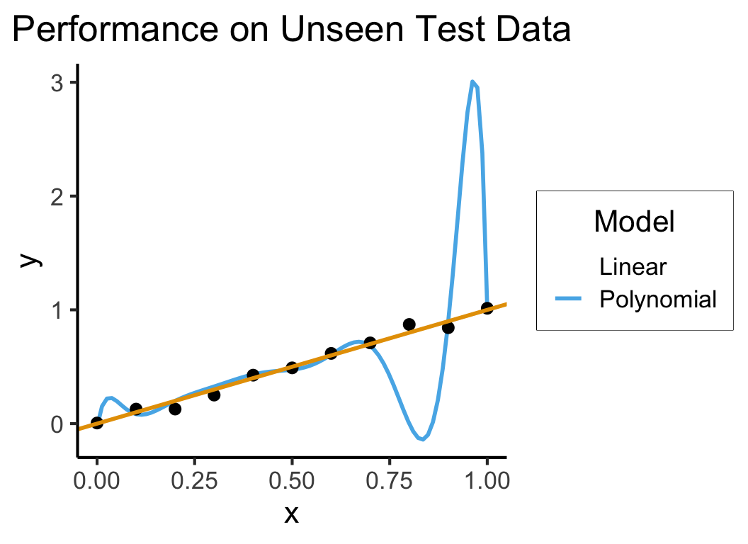
Training vs. Test Data

Cross-Validation

• The idea that good models generalize well is crucial!
  • What if we could leverage this insight to optimize over our training data?
  • The key: Validation Sets

Hyperparameters

• The unspoken (but highly consequential!) “settings” for our learning procedure (that we haven’t optimized via gradient descent)
• There are several we’ve already seen – can you name them?

• Unsupervised Clustering: The number of clusters we want (\(K\))
• Gradient Descent: The step size \(\gamma\)
• LASSO/Elastic Net: \(\lambda\)
• The train/validation/test split!

Hyperparameter Selection

• Every model comes with its own hyperparameters:
  • Neural Networks: Number of layers, number of nodes per layer
  • Decision Trees: Maximum tree depth, max number of features to include
  • Topic Models: Number of topics, document/topic priors
• So, how do we choose?
  • Often more art than science
  • Principled, universally applicable, but slow: grid search
  • Specific methods for specific algorithms: ADAM [@kingma_adam_2017] for Neural Network learning rates)

Appendix: Harmonic Mean

• \(\mathsf{HMean}\) is the harmonic mean, an alternative to the standard (arithmetic) mean
• Penalizes greater “gaps” between precision and recall: if precision is 0 and recall is 1, for example, their arithmetic mean is 0.5 while their harmonic mean is 0.
• For the curious: given numbers \(X = \{x_1, \ldots, x_n\}\), \(\mathsf{HMean}(X) = \frac{n}{\sum_{i=1}^nx_i^{-1}}\)