Week 3: Getting Fancy with Regression
DSAN 5300: Statistical Learning
Spring 2025, Georgetown University
Monday, January 27, 2025
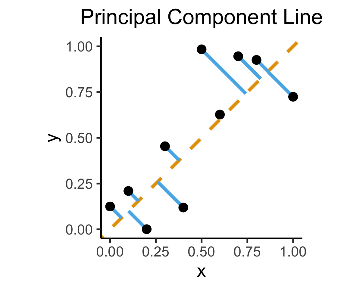
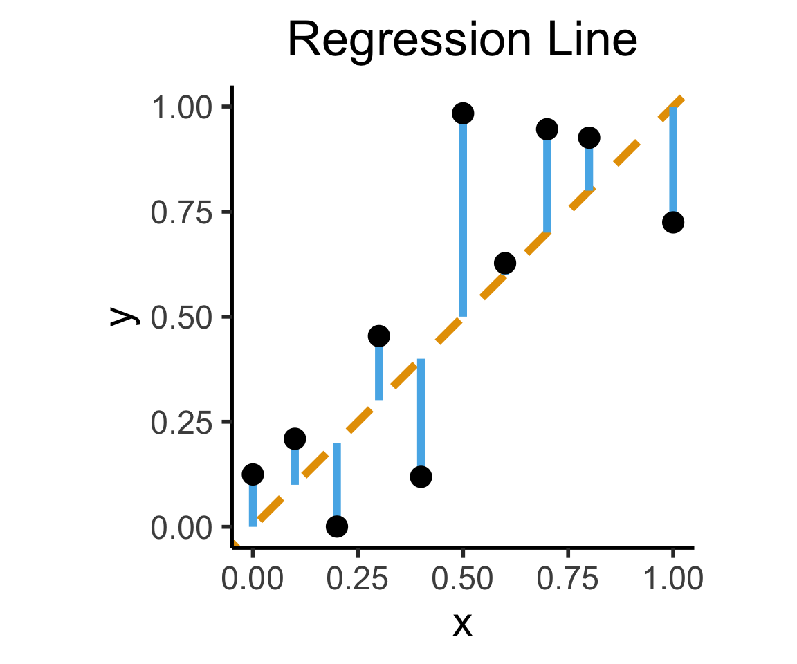
How Do We Define “Best”?
- Intuitively, two different ways to measure how well a line fits the data:
Code
library(tidyverse)
set.seed(5321)
N <- 11
x <- seq(from = 0, to = 1, by = 1 / (N - 1))
y <- x + rnorm(N, 0, 0.2)
mean_y <- mean(y)
spread <- y - mean_y
df <- tibble(x = x, y = y, spread = spread)
ggplot(df, aes(x=x, y=y)) +
  geom_abline(slope=1, intercept=0, linetype="dashed", color=cbPalette[1], linewidth=g_linewidth*2) +
  geom_segment(xend=(x+y)/2, yend=(x+y)/2, linewidth=g_linewidth*2, color=cbPalette[2]) +
  geom_point(size=g_pointsize) +
  coord_equal() +
  xlim(0, 1) + ylim(0, 1) +
  dsan_theme("half") +
  labs(
    title = "Principal Component Line"
  )
ggplot(df, aes(x=x, y=y)) +
  geom_abline(slope=1, intercept=0, linetype="dashed", color=cbPalette[1], linewidth=g_linewidth*2) +
  geom_segment(xend=x, yend=x, linewidth=g_linewidth*2, color=cbPalette[2]) +
  geom_point(size=g_pointsize) +
  coord_equal() +
  xlim(0, 1) + ylim(0, 1) +
  dsan_theme("half") +
  labs(
    title = "Regression Line"
  )
Visualizing Multiple Linear Regression

(ISLR, Fig 3.5): A pronounced non-linear relationship. Positive residuals (visible above the surface) tend to lie along the 45-degree line, where budgets are split evenly. Negative residuals (most not visible) tend to be away from this line, where budgets are more lopsided.
Another MLR Superpower: Incorporating Categorical Vars
\[ \begin{align*} Y &= \beta_0 + \beta_1 \times \texttt{income} \\ &\phantom{Y} \end{align*} \]
Code
credit_df <- read_csv("assets/Credit.csv")
credit_plot <- credit_df |> ggplot(aes(x=Income, y=Balance)) +
  geom_point(size=0.5*g_pointsize) +
  geom_smooth(method='lm', formula="y ~ x", linewidth=1) +
  theme_dsan() +
  labs(
    title="Credit Card Balance vs. Income Level",
    x="Income ($1K)",
    y="Credit Card Balance ($)"
  )
credit_plot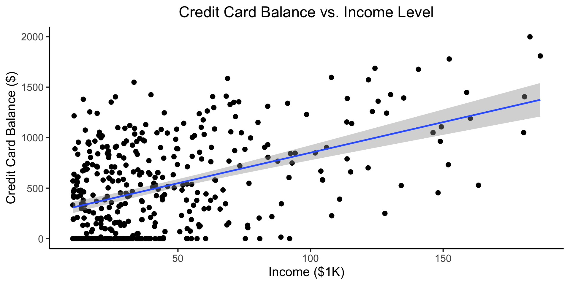
\[ \begin{align*} Y = &\beta_0 + \beta_1 \times \texttt{income} + \beta_2 \times \texttt{Student} \\ &+ \beta_3 \times (\texttt{Student} \times \texttt{Income}) \end{align*} \]
Code
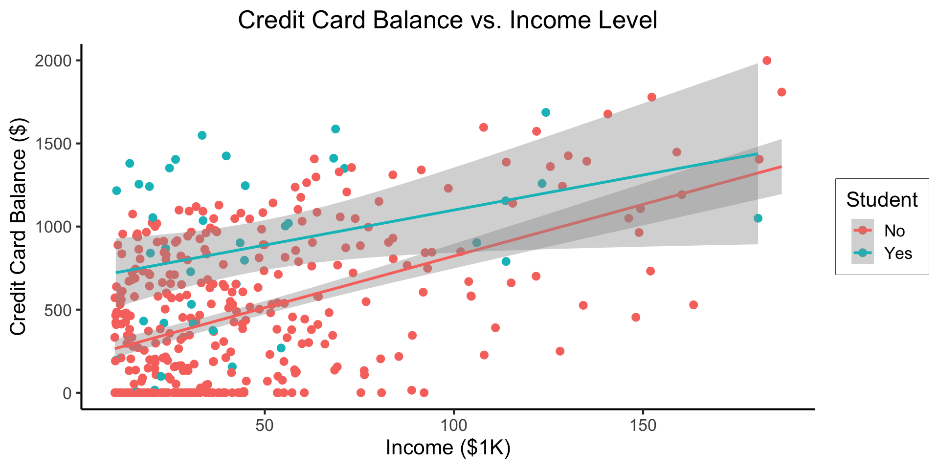
- Why do we need the \(\texttt{Student} \times \texttt{Income}\) term?
- Understanding this setup will open up a vast array of possibilities for regression 😎
- (Dear future Jeff, let’s go through this on the board! Sincerely, past Jeff)
From MLR to Logistic Regression
- As DSAN students, you know that we’re still sweeping classification under the rug!
- We saw how to include binary/multiclass covariates, but what if the actual thing we’re trying to predict is binary?
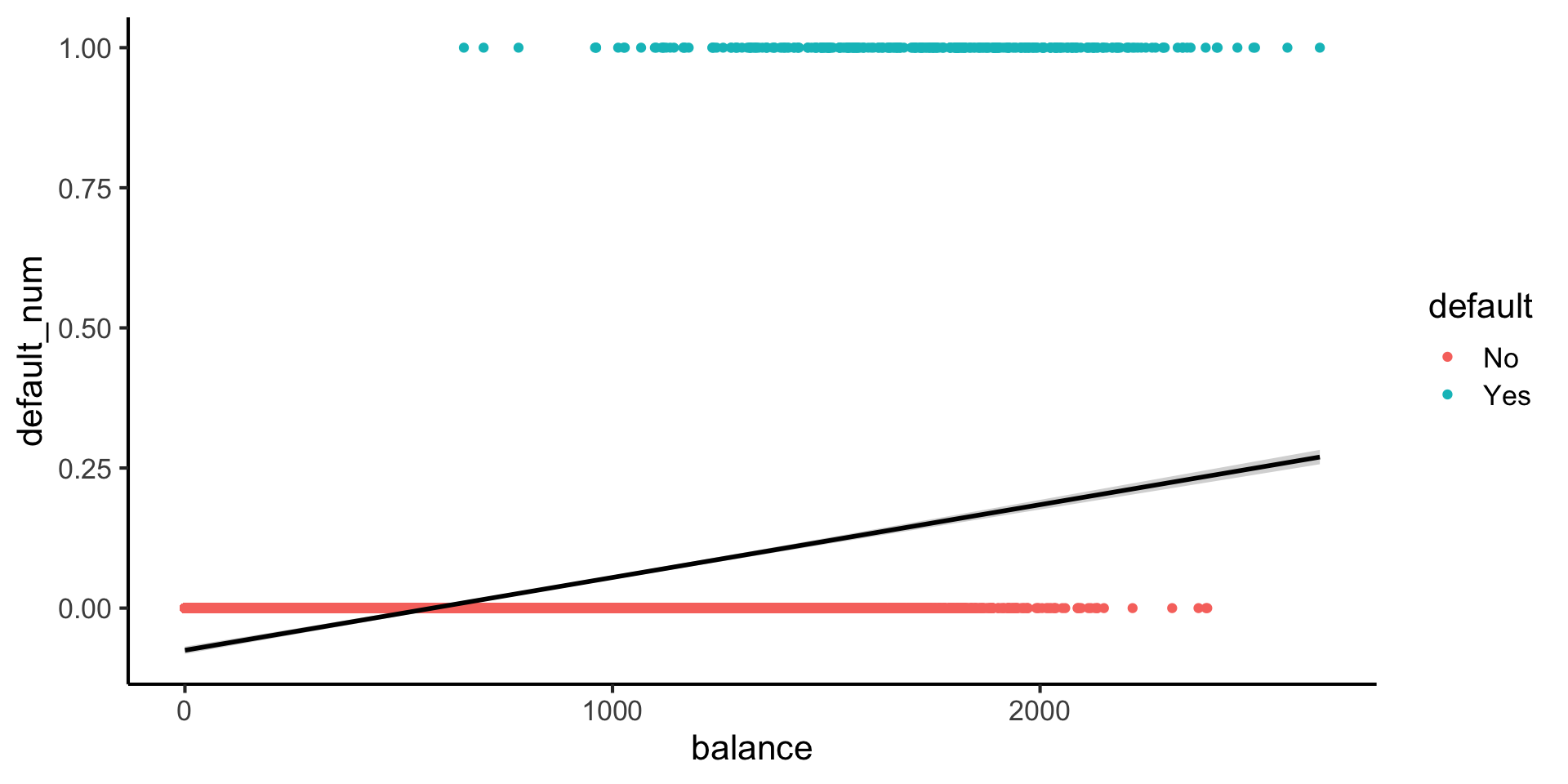
- The wrong approach is the “Linear Probability Model”:
\[ \Pr(Y \mid X) = \beta_0 + \beta_1 X + \varepsilon \]

Credit Default
Code
library(tidyverse)
library(ggExtra)
default_df <- read_csv("assets/Default.csv") |>
  mutate(default_num = ifelse(default=="Yes",1,0))
default_plot <- default_df |> ggplot(aes(x=balance, y=income, color=default, shape=default)) +
  geom_point(alpha=0.6) +
  theme_classic(base_size=16) +
  labs(
    title="Credit Defaults by Income and Account Balance",
    x = "Account Balance",
    y = "Income"
  )
default_mplot <- default_plot |> ggMarginal(type="boxplot", groupColour=FALSE, groupFill=TRUE)
default_mplot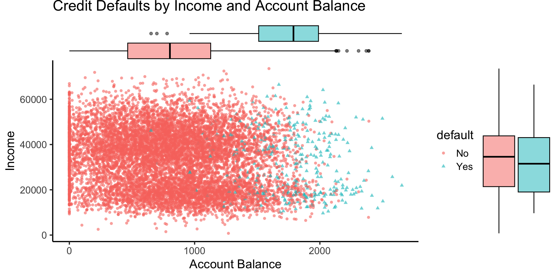
Lines vs. Sigmoids(!)
Here’s what lines look like for this dataset:
Here’s what sigmoids look like:
Code
library(tidyverse)
logistic_model <- glm(default_num ~ balance, family=binomial(link='logit'),data=default_df)
default_df$predictions <- predict(logistic_model, newdata = default_df, type = "response")
my_sigmoid <- function(x) 1 / (1+exp(-x))
default_df |> ggplot(aes(x=balance, y=default_num)) +
  #stat_function(fun=my_sigmoid) +
  geom_point(aes(color=default)) +
  geom_line(
    data=default_df,
    aes(x=balance, y=predictions),
    linewidth=1
  ) +
  theme_classic(base_size=16)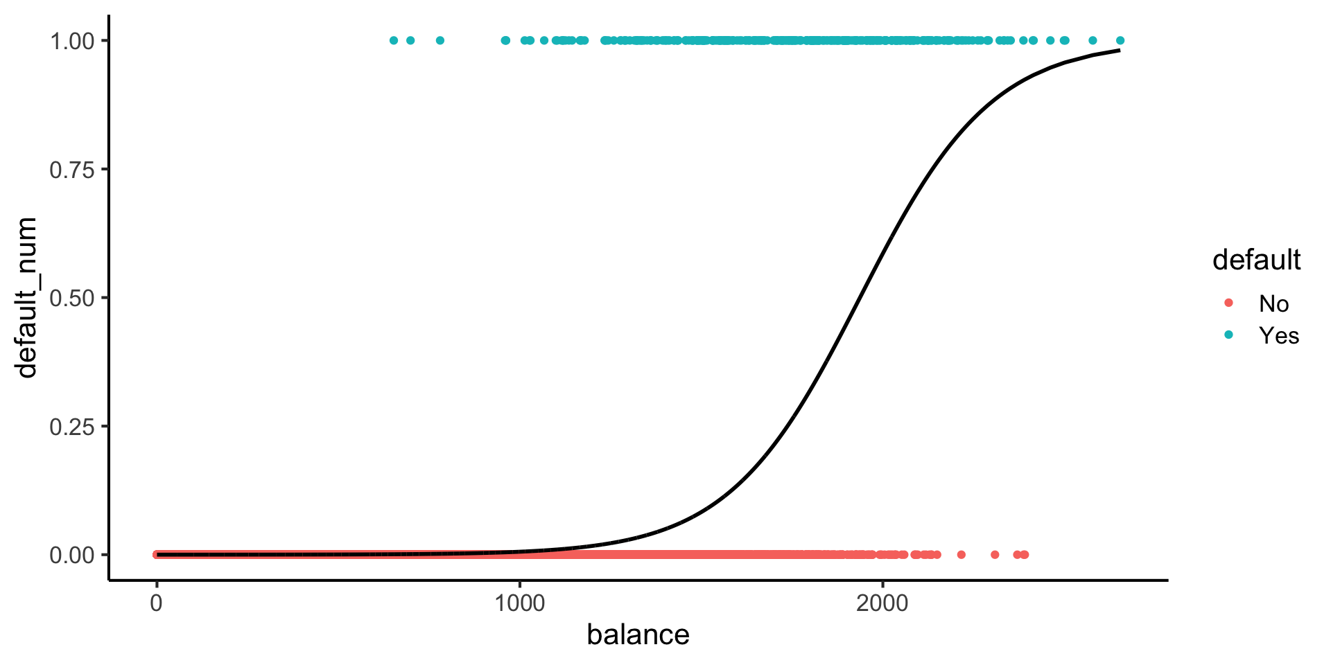
\[ \Pr(Y \mid X) = \beta_0 + \beta_1 X + \varepsilon \]
\[ \log\underbrace{\left[ \frac{\Pr(Y \mid X)}{1 - \Pr(Y \mid X)} \right]}_{\mathclap{\smash{\text{Odds Ratio}}}} = \beta_0 + \beta_1 X + \varepsilon \]