Week 12: Non-Parametric Statistics

DSAN 5100: Probabilistic Modeling and Statistical Computing
Section 01

Class Sessions

Author

Purna Gamage, Amineh Zadbood, and Jeff Jacobs

Published

Tuesday, November 18, 2025

Open slides in new window →

Non-Parametric Statistics: Overview

How is Non-Parametric Different from What We’ve Been Doing?

Statistical models and hypothesis tests we’ve learned thus far were parametric
Meaning: Assume population follows this distribution, then estimate population parameters (e.g., \(\param{\mu}\) and \(\param{\sigma}\)) using MLE, GMM, etc.

What Makes It “Non-Parametric”?

We’ve talked about how the Normal distribution is “standard” in multiple senses:
- Empirically: It arises from common processes in nature, like random walks
- Theoretically: It is the maximum-entropy distribution which encodes only¹ knowledge of a mean \(\mu\) and a variance \(\sigma^2\)
Then we talked about estimating these parameters (\(\param{\mu}\) and \(\param{\sigma^2}\)) from data: different ways to amalgamate information from an observed sample \(\mathbf{X} = (X_1, \ldots, X_n)\) to estimate (unobserved) \(\param{\mu}\) and \(\param{\sigma}^2\) with minimal bias and variance

We therefore “funnel” all of the information contained in \(\mathbf{X}\) down into estimates of \(\param{\mu}\) and \(\param{\sigma^2}\)
But… what if we’re wrong? What if the DGP is not based on a Normal distribution?

What If We’re Wrong?

It is this concern: the fact that all of our results, all of our confidence about our estimates thus far, come as a result of making distributional assumptions
Non-parametric analysis tries to avoid this potential catastrophe by making as few distributional assumptions as possible
Recall how parameters of a distribution determine all information you could possibly want to know about the distribution (via Moment Generating Function):

Type of Distribution	+	Parameter Values	=	All Possible Info (MGF)
Normal \(~\mathcal{N}(\param{\mu}, \param{\sigma^2})\)	+	\(\param{\mu} = m\), \(\param{\sigma^2} = s^2\)	=	\(M_t(X) = \exp[mt + s^2t^2/2]\)
Uniform \(~\mathcal{U}(\param{\alpha},\param{\beta})\)	+	\(\param{\alpha} = a\), \(\param{\beta} = b\)	=	\(M_t(X) = \frac{e^{tb} - e^{ta}}{t(b-a)}\)
Poisson \(~\text{Pois}(\param{\lambda})\)	+	\(\param{\lambda} = \ell\)	=	\(M_t(X) = \exp[\ell(e^t - 1)]\)

Avoiding Wrongness Disasters: The Sign Test

Sign Test Intuition

Instead of trying to estimate all possible info about the underlying distribution, we only estimate one piece of information that we need to test a hypothesis
Example: for populations \(\chi\), \(\psi\), if \(H_A: \mu_\chi > \mu_\psi\), skip intermediate step of estimating distributions \(\mathcal{D}_\chi(\param{\theta})\), \(\mathcal{D}_\psi(\param{\theta})\) from samples \(\mathbf{X}\), \(\mathbf{Y}\)!
Instead, just directly “extract” greater than vs. not greater than info from \(\mathbf{X}\) and \(\mathbf{Y}\) (median \(m\) always exists as “pivot” for well-behaved \(X\), \(\Pr(X > m) = 0.5\))
It will help us to define \(\text{Sign}(x) = \begin{cases}\phantom{-}1 &\text{if } x > 0 \\ \phantom{-}0 &\text{if }x = 0 \\ -1 &\text{if }x < 0\end{cases}\)
If \(\mathbf{X} = (15, 7, 11, 3)\), \(\mathbf{Y} = (-3, 4, 1, 4)\), we can compute a “greater-than score”:

\[ \begin{align*} \sum_{i=1}^N \sign(X_i - Y_i) &= \sign(15 - (-3)) + \sign(7-4) + \sign(11-1) + \sign(3-4) \\ &= 1 + 1 + 1 + -1 = 2 \end{align*} \]

So long as slots are comparable (notice \(\mathbf{X}, \mathbf{Y}\) are ordered), we can compare this with \(0\), our expectation if \(\chi = \psi\), regardless of underlying distributions \(\mathcal{D}_\chi, \mathcal{D}_\psi\).

Procedure in General

\(\mathbf{X}\): size-\(N\) sample from population \(\chi\); \(\mathbf{Y}\): size-\(N\) sample from population \(\psi\)
(Rather than estimating \(\mathcal{D}_\chi\) from \(\mathbf{X}\) and \(\mathcal{D}_\psi\) from \(\mathbf{Y}\)), we directly pair datapoints \(X_i \in \mathbf{X}\) and \(Y_i \in \mathbf{Y}\) and compute the sign of their difference:

\[ \text{GT}_i(X_i, Y_i) = \text{Sign}(X_{i} - Y_{i}) = \begin{cases} \phantom{-}1 &\text{if }X_{i} > Y_{i}, \\ \phantom{-}0 &\text{if }X_{i} = Y_{i}, \\ -1 &\text{if }X_{i} < Y_{i} \end{cases} \]

We can then sum each pair’s score into an aggregate score:

\[ \text{GT}(\mathbf{X}, \mathbf{Y}) = \sum_{i=1}^NGT_i(X_i,Y_i) \]

such that if \(\chi\) and \(\psi\) are in fact the same population, we expect \(GT(\mathbf{X}, \mathbf{Y}) = 0\) (positive and negative values of \(GT_i\) cancel each other out, for sufficiently large \(N\))
Non-parametric tests which use this value as a test statistic are called Sign tests

Mann-Whitney U Test: Paired Observations → Paired Samples

Also called the Wilcoxon Rank Sum Test

What If We Can’t Pair Observations One-to-One?

For example, what if samples aren’t the same size: \(N_X = |\mathbf{X}| \neq N_Y = |\mathbf{Y}|\)?
Intuition: If there is no “natural” one-to-one pairing of the observations, we can instead consider all possible pairs \((X_{i}, Y_{j}) \in \mathbf{X} \times \mathbf{Y}\)
We can then count how often \(X_i > Y_j\), how often \(Y_j > X_i\), and compare this to our expectation of how often these would occur if \(\chi = \psi\) (that is, if \(\mathbf{X}\) and \(\mathbf{Y}\) were in fact drawn from the same population)

Computational Efficiency

We could just go ahead with this intuition, checking every pair and seeing how often \(X_i > Y_j\) vs. how often \(Y_j > X_i\), but this is computationally expensive for large samples (requiring \(O(N_1N_2)\) comparisons)
So, let’s walk through an example with pairwise comparisons, but try to think of an equivalent yet sub-quadratic method for achieving the same results!

Pairwise Comparison Mode

Let \(\mathbf{X} = \{5, 9, 7\}, \mathbf{Y} = \{7, 6\}\), and consider \(X_i > Y_j\) vs. \(Y_j > X_i\) for all pairs:
Give 1 point to \(\mathbf{X}\) if \(X_i > Y_j\), 1 point to \(\mathbf{Y}\) if \(Y_j > X_i\), 0.5 points to both if \(X_i = Y_j\).

\(X_i\)	\(Y_j\)	\(>\)	\(=\)	\(<\)
5	7			+1
5	6			+1
9	7	+1
9	6	+1
7	7		+0.5
7	6	+1
Final	Score:	\(S_{\mathbf{X}} = 3.5\)		\(S_{\mathbf{Y}} = 2.5\)

Ranking Mode

Now consider the combined dataset \(\mathbf{Z} = \mathbf{X} \oplus \mathbf{Y} = (5_X, 9_X, 7_X, 7_Y, 6_Y)\)
Let’s see what we get when we rank the values in \(\mathbf{X}\) and \(\mathbf{Y}\) separately, then rank the same values within \(\mathbf{Z}\), keeping track of whether each number is from \(\mathbf{X}\) or \(\mathbf{Y}\):

Values	\(5_X\)	\(6_Y\)	\(7_X\)	\(7_Y\)	\(9_X\)
Rank in \(\mathbf{X}\)	\([1]_{X/\mathbf{X}}\)		\([2]_{X/\mathbf{X}}\)		\([3]_{X/\mathbf{X}}\)	\(\Sigma_{X/\mathbf{X}} = [6]\)
Rank in \(\mathbf{Y}\)		\([1]_{Y/\mathbf{Y}}\)		\([2]_{Y/\mathbf{Y}}\)		\(\Sigma_{Y/\mathbf{Y}} = [3]\)
Rank in \(\mathbf{Z}\)	\([1]_{X/\mathbf{Z}}\)	\([2]_{Y/\mathbf{Z}}\)	\([3.5]_{X/\mathbf{Z}}\)	\([3.5]_{Y/\mathbf{Z}}\)	\([5]_{X/\mathbf{Z}}\)	\(\Sigma_{X/\mathbf{Z}} = [9.5]\) \(\Sigma_{Y/\mathbf{Z}} = [5.5]\)

Thus, by subtracting single-sample ranks from combined-sample ranks, we obtain:
\(S_{\mathbf{X}} = \Sigma_{X/\mathbf{Z}} - \Sigma_{X/\mathbf{X}} = 9.5 - 6 = 3.5\)
\(S_{\mathbf{Y}} = \Sigma_{Y/\mathbf{Z}} - \Sigma_{Y/\mathbf{Y}} = 5.5 - 3 = 2.5\) 🤯
And yet, this runs in \(O((N_1+N_2)\log(N_1+N_2)) < O(N_1N_2)\)

Example: 2022 World Cup

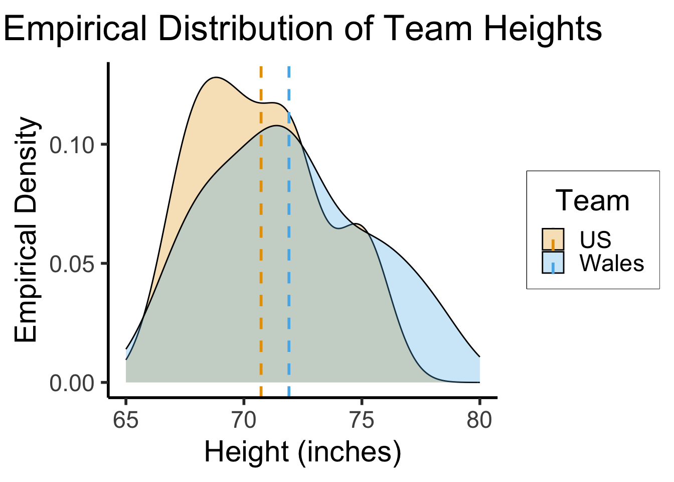
Heights (inches) of Welsh vs. US national football teams (\(N = 22\) players total):

Wales	78	71	76	75	72	70	68	72	69	73	67	\(\overline{X} \approx 71.91\)
USA	75	68	75	69	70	70	72	67	72	72	70	\(\overline{Y} \approx 70.73\)

Code

library(tidyverse)
# Manual (via tibble)
# us_heights <- tibble(height=c(75, 68, 74, 68, 68, 70, 72, 67, 72, 72, 70))
# corrected
us_heights <- tibble(height=c(75, 68, 75, 69, 70, 70, 72, 67, 72, 72, 68))
mean_us <- mean(us_heights$height)
us_heights <- us_heights |> mutate(Team = "US")
wales_heights <- tibble(height=c(78, 71, 76, 75, 72, 70, 68, 72, 69, 73, 67))
mean_wales <- mean(wales_heights$height)
# From csv
# https://www.fifa.com/en/match-centre/match/17/255711/285063/400235455
team_df <- read_csv("assets/wc_usa_wales.csv")
# team_df |> group_by(team) |> summarize(height_mean = mean(height_in))
mean_df <- tibble(mean_height = c(mean_us, mean_wales), Team = c("US", "Wales"))
wales_heights <- wales_heights |> mutate(Team = "Wales")
players = bind_rows(us_heights, wales_heights)
ggplot(players, aes(x=height, fill=Team)) +
  geom_density(
    alpha=0.3, adjust=4/5
  ) +
  geom_vline(
    data=mean_df,
    aes(xintercept=mean_height, color=Team),
    linetype = "dashed",
    linewidth = g_linewidth
  ) +
  xlim(c(65,80)) +
  dsan_theme("half") +
  scale_fill_manual(values=c(cbPalette[1], cbPalette[2])) +
  labs(
    title = "Empirical Distribution of Team Heights",
    x = "Height (inches)",
    y = "Empirical Density"
  )

Samples \(\rightarrow\) Populations

We know that the sampled heights of Welsh football players (\(\mathbf{X}\)) are (on average) greater than the sampled heights of US football players (\(\mathbf{Y}\)).
But are heights in fact greater among the population of Welsh football players (\(\chi\)), relative to the population of US football players (\(\psi\))?

The Non-Parametric Fork in the Road

Recall: in parametric tests, when comparing means, we analyzed the difference in the sample means relative to their variability and summarized the sample information in a test statistic: for example, \(t = \frac{\overline{X} - \mu_H}{\widehat{\sigma} / \sqrt{N}}\)
We could compute this test statistic, but it would implicitly depend on an assumption of the underlying DGP: that heights follow a Normal distribution.
Here, instead, we produce a test statistic based on the ranks!
Test statistics should measure how surprised we would be if we observed what we observed in a world where the null hypothesis is true
Equivalently, it should be low if the observed difference could feasibly have occurred just due to random noise (i.e., if we’re looking at noisy data from world where null hypothesis is true)
So, let’s think in these terms about the ranks of each datapoint, to develop a non-parametric test statistic based on the ranks

Choosing Non-Parametric Hypotheses

The empirical distributions from the previous slide, and the small sample size (\(N_1 = N_2 = 11\)), motivate our use of a nonparametric test!
Assuming \(X \sim \mathcal{D}_1\) and \(Y \sim \mathcal{D}_2\) (but not assuming the parametric forms of \(\mathcal{D}_1\) or \(\mathcal{D}_2\)!), we can test:
\(H_0: \Pr(X > Y) = \Pr(Y > X)\)
\(H_1: \Pr(X > Y) \neq \Pr(Y > X)\)

Sorting and Ranking Observations

Original Data		Sorted Total Samples		Rank
USA	Wales	USA	Wales	USA	Wales
75	78	67	67	1.5	1.5
68	71	68	68	4	4
75	76	68	68	4	4
69	75	69	69	6.5	6.5
70	72	70	70	9	9
70	70	70	70	9	9
72	68		71		11
67	72	72	72	14	14
67	72	72		14
72	69	72		14
72	69	72	72	14	14
72	73	72		14
72	73	72		14
68	67		73		17
		75	75	19	19
		75	75	19	19
			76		21
			78		22

Our Rank-Based Test Statistic

Sums of ranks relative to the combined dataset: \(\Sigma_{X/\mathbf{Z}} = 112.5\), \(\Sigma_{Y/\mathbf{Z}} = 140.5\).
And then sum the ranks in each group, relative to the same group… In general, if we have \(N\) ranked datapoints (so, datapoints given labels \(\{1, 2, \ldots, N\}\)), what will the sum of these individual ranks be?

\[ \sum_{i=1}^{N}i = \underbrace{\overbrace{(1 + N)}^{N + 1} + \overbrace{(2 + (N-1))}^{N + 1} + \cdots}_{N/2\text{ terms}} = \frac{N(N+1)}{2} \]

So, in this case,

\[ \Sigma_{X/\mathbf{X}} = \Sigma_{Y/\mathbf{Y}} = \sum_{i=1}^{11}i = \frac{11(12)}{2} = 66 \]

Giving us the test statistics

\[ \begin{align*} U_X &= 112.5 - 66 = 46.5, \; U_Y = 140.5 - 66 = 74.5 \\ U &= \min\{U_X, U_Y\} = \min\{46.5, 74.5\} = 46.5 \end{align*} \]

Simulating (One) Null-Hypothesis World

One simulation:

set.seed(5100)
library(tidyverse)
N1 <- 11
N2 <- 11
N <- N1 + N2
totalRankSum <- (N * (N+1)) / 2
s_1 <- runif(N1)
df_1 <- tibble(x = s_1, team = "A")
s_2 <- runif(N2)
df_2 <- tibble(x = s_2, team = "B")
df_combined <- bind_rows(df_1, df_2)
df_combined['rank'] <- rank(df_combined$x)
writeLines(paste0("N1 = ",N1,", N2 = ",N2," => Sum(1...(N1+N2)) = ",totalRankSum))

N1 = 11, N2 = 11 => Sum(1...(N1+N2)) = 253

df_combined |> arrange(rank) |> head()

x	team	rank
0.0281644	B	1
0.0282184	A	2
0.0730575	B	3
0.1343398	B	4
0.1351495	B	5
0.1858087	A	6

→

df_combined |> group_by(team) |> summarize(ranksum = sum(rank)) |> mutate(proportion = ranksum / totalRankSum)

team	ranksum	proportion
A	144	0.56917
B	109	0.43083

Simulating Many Null-Hypothesis Worlds

And we can repeat this process (say) 10K times:

simulate_ranksums <- function(N1, N2) {
  N <- N1 + N2
  totalRankSum <- (N * (N+1)) / 2
  s_1 <- runif(N1)
  df_1 <- tibble(x = s_1, team = "A")
  s_2 <- runif(N2)
  df_2 <- tibble(x = s_2, team = "B")
  df_combined <- bind_rows(df_1, df_2)
  df_combined['rank'] <- rank(df_combined$x)
  ranksum_df <- df_combined |> group_by(team) |> summarize(ranksum = sum(rank))
  return(ranksum_df$ranksum)
}
num_sims <- 1000
results <- replicate(num_sims, simulate_ranksums(11,11))
t(results[,0:10])

      [,1] [,2]
 [1,]  133  120
 [2,]   98  155
 [3,]  115  138
 [4,]  166   87
 [5,]  137  116
 [6,]  140  113
 [7,]  146  107
 [8,]  157   96
 [9,]  119  134
[10,]  106  147

rowMeans(results)

[1] 126.407 126.593

# Separate ranksums
ranksum_A <- tibble(ranksum=results[1,], team="A")
ranksum_A_mean <- mean(ranksum_A$ranksum)
ranksum_B <- tibble(ranksum=results[2,], team="B")
ranksum_B_mean <- mean(ranksum_B$ranksum)
sim_df <- bind_rows(ranksum_A, ranksum_B)
# Means
mean_df <- tibble(mean_value = c(ranksum_A_mean, ranksum_B_mean), team=c("A","B"))
mean_center <- (ranksum_A_mean + ranksum_B_mean) / 2
gen_ranksum_plot <- function(radius=Inf) {
  ranksum_plot <- ggplot(sim_df, aes(x=ranksum, fill=team)) +
    geom_density(linewidth = g_linewidth, alpha=0.333) +
    geom_vline(
        data=mean_df,
        aes(xintercept = mean_value, color=team),
        linewidth = g_linewidth
    ) +
    theme_classic(base_size=14) +
    scale_fill_manual(values=c(cbPalette[1], cbPalette[2]))
    if (radius != Inf) {
        ranksum_plot <- ranksum_plot +
        xlim(mean_center - radius, mean_center + radius)
    }
    return(ranksum_plot)
}
gen_ranksum_plot()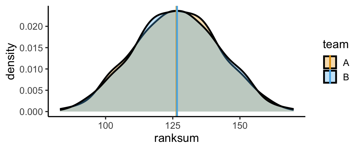

gen_ranksum_plot(radius=8)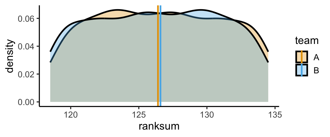

`wilcox.test` in R