Week 8: Supervised and Unsupervised Learning
DSAN 5000: Data Science and Analytics
Thursday, October 24, 2024
Machine Learning
\[ \DeclareMathOperator*{\argmax}{argmax} \DeclareMathOperator*{\argmin}{argmin} \newcommand{\bigexp}[1]{\exp\mkern-4mu\left[ #1 \right]} \newcommand{\bigexpect}[1]{\mathbb{E}\mkern-4mu \left[ #1 \right]} \newcommand{\definedas}{\overset{\text{defn}}{=}} \newcommand{\definedalign}{\overset{\phantom{\text{defn}}}{=}} \newcommand{\eqeventual}{\overset{\text{eventually}}{=}} \newcommand{\expect}[1]{\mathbb{E}[#1]} \newcommand{\expectsq}[1]{\mathbb{E}^2[#1]} \newcommand{\fw}[1]{\texttt{#1}} \newcommand{\given}{\mid} \newcommand{\green}[1]{\color{green}{#1}} \newcommand{\heads}{\outcome{heads}} \newcommand{\lik}{\mathcal{L}} \newcommand{\mle}{\textsf{ML}} \newcommand{\orange}[1]{\color{orange}{#1}} \newcommand{\outcome}[1]{\textsf{#1}} \newcommand{\param}[1]{{\color{purple} #1}} \newcommand{\paramDist}{\param{\boldsymbol\theta_\mathcal{D}}} \newcommand{\pgsamplespace}{\{\green{1},\green{2},\green{3},\purp{4},\purp{5},\purp{6}\}} \newcommand{\prob}[1]{P\left( #1 \right)} \newcommand{\purp}[1]{\color{purple}{#1}} \newcommand{\spacecap}{\; \cap \;} \newcommand{\spacewedge}{\; \wedge \;} \newcommand{\tails}{\outcome{tails}} \newcommand{\Var}[1]{\text{Var}[#1]} \newcommand{\bigVar}[1]{\text{Var}\mkern-4mu \left[ #1 \right]} \]
Supervised vs. Unsupervised Learning
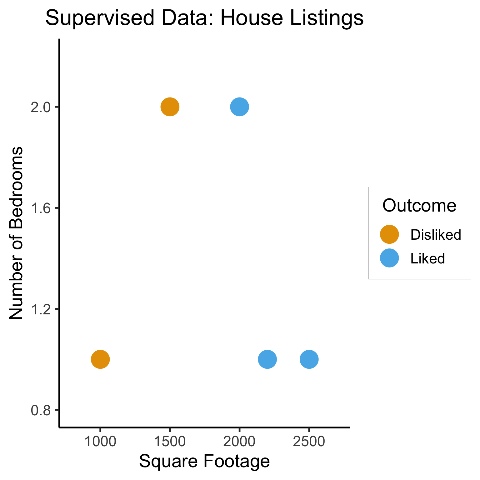
Supervised Learning: You want the computer to learn the existing pattern of how you are classifying1 observations
- Discovering the relationship between properties of data and outcomes
- Example (Binary Classification): I look at homes on Zillow, saving those I like to folder A and don’t like to folder B
- Example (Regression): I assign a rating of 0-100 to each home
- In both cases: I ask the computer to learn my schema (how I classify)
Unsupervised Learning: You want the computer to find patterns in a dataset, without any prior classification info
- Typically: grouping or clustering observations based on shared properties
- Example (Clustering): I save all the used car listings I can find, and ask the computer to “find a pattern” in this data, by clustering similar cars together
Dataset Structures
Supervised Learning: Dataset has both explanatory variables (“features”) and response variables (“labels”)
Code
| home_id | sqft | bedrooms | rating |
|---|---|---|---|
| 0 | 1000 | 1 | Disliked |
| 1 | 2000 | 2 | Liked |
| 2 | 2500 | 1 | Liked |
| 3 | 1500 | 2 | Disliked |
| 4 | 2200 | 1 | Liked |
Dataset Structures: Visualized
Code
library(tidyverse)
# To force a legend
unsup_grouped <- unsup_data |> mutate(big=bedrooms > 1)
unsup_grouped[['big']] <- factor(unsup_grouped[['big']], labels=c("?1","?2"))
ggplot(unsup_grouped, aes(x=sqft, y=bedrooms, fill=big)) +
  geom_point(size = g_pointsize * 2) +
  labs(
    x = "Square Footage",
    y = "Number of Bedrooms",
    fill = "?"
  ) +
  dsan_theme("half") +
  expand_limits(x=c(800,2700), y=c(0.8,2.2)) +
  ggtitle("Unsupervised Data: House Listings") +
  theme(legend.background = element_rect(fill="white", color="white"), legend.box.background = element_rect(fill="white"), legend.text = element_text(color="white"), legend.title = element_text(color="white"), legend.position = "right") +
  scale_fill_discrete(labels=c("?","?")) +
  #scale_color_discrete(values=c("white","white"))
  scale_color_manual(name=NULL, values=c("white","white")) +
  #scale_color_manual(values=c("?1"="white","?2"="white"))
  guides(fill = guide_legend(override.aes = list(shape = NA)))
Different Goals
Code
ggplot(sup_data, aes(x=sqft, y=bedrooms, color=rating)) +
  geom_point(size = g_pointsize * 2) +
  labs(
    title = "Supervised Data: House Listings",
    x = "Square Footage",
    y = "Number of Bedrooms",
    color = "Outcome"
  ) +
  dsan_theme("half") +
  expand_limits(x=c(800,2700), y=c(0.8,2.2)) +
  geom_vline(xintercept = 1750, linetype="dashed", color = "black", size=1) +
  annotate('rect', xmin=-Inf, xmax=1750, ymin=-Inf, ymax=Inf, alpha=.2, fill=cbPalette[1]) +
  annotate('rect', xmin=1750, xmax=Inf, ymin=-Inf, ymax=Inf, alpha=.2, fill=cbPalette[2])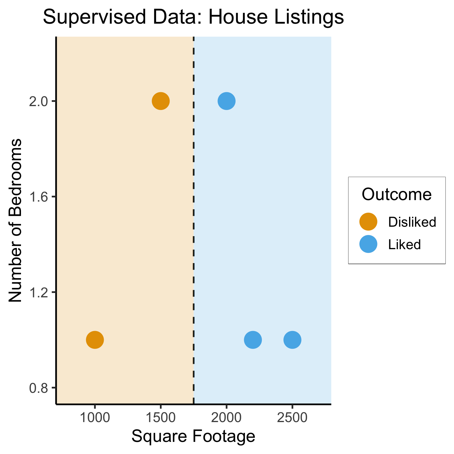
Code
library(ggforce)
ggplot(unsup_grouped, aes(x=sqft, y=bedrooms)) +
  #scale_color_brewer(palette = "PuOr") +
  geom_mark_ellipse(expand=0.1, aes(fill=big), size = 1) +
  geom_point(size=g_pointsize) +
  labs(
    x = "Square Footage",
    y = "Number of Bedrooms",
    fill = "?"
  ) +
  dsan_theme("half") +
  ggtitle("Unsupervised Data: House Listings") +
  #theme(legend.position = "none") +
  #theme(legend.title = text_element("?"))
  expand_limits(x=c(800,2700), y=c(0.8,2.2)) +
  scale_fill_manual(values=c(cbPalette[3],cbPalette[4]), labels=c("?","?"))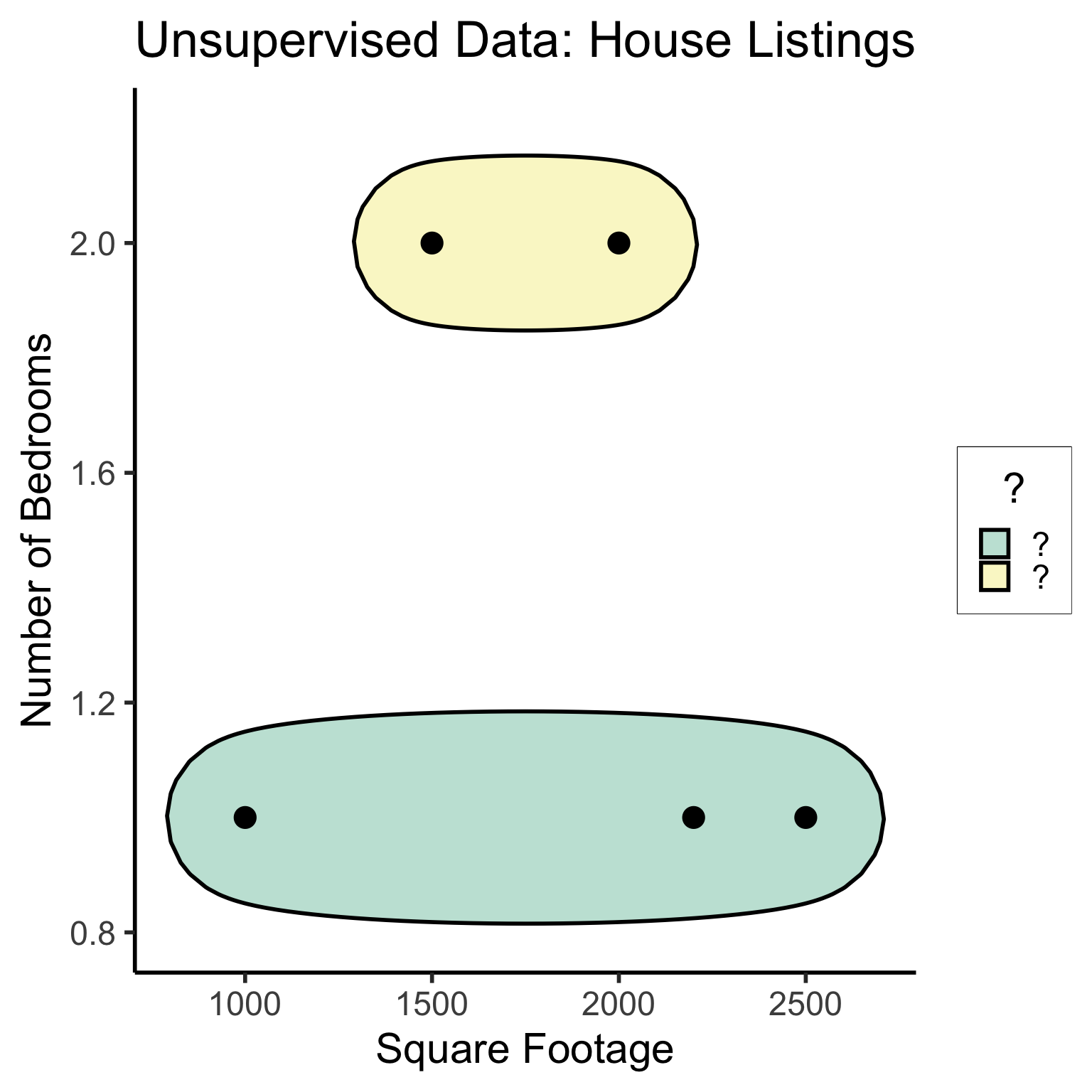
K-Nearest Neighbors (KNN)
The KNN Algorithm
- Binary Classification: Given a set of information (“features”) about an observation (\(X\)), predict a yes/no outcome (\(y \in \{0, 1\}\)) for this observation
- Example: Given a count of words in an email, classify it as spam (\(y=1\)) or not spam (\(y = 0\))
- Multiclass classification: Classify the observation into one of \(N\) categories (\(y \in \{0, 1, \ldots, N\}\))
- Example: Given a handwritten symbol, classify it as a digit (\(y = \{0, 1, \ldots, 9\}\))
- K-Nearest Neighbors Intuition: Find the \(K\) most similar observations that we’ve seen before, and have them “majority vote” on the outcome.
MNIST Digits Example
KNN Example
- The problem: Given a student’s GPA, predict whether or not they will graduate
- K-Nearest Neighbor Approach:
- Get a dataset of previous years, students’ GPAs and whether or not they graduated
- Find the \(K = 5\) students with GPA closest to the student of interest
- If a majority of these 5 students graduated, predict that the student will graduate. Otherwise, predict that they will not.
KNN In Pictures
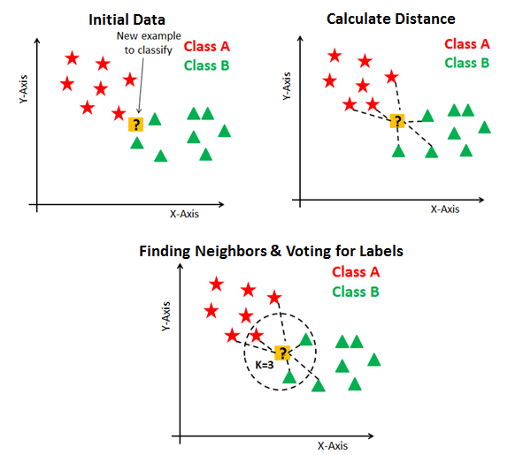
Image credit: DataCamp tutorial
Naïve Bayes Classifiers
What is “Naïve” About It?
Guessing House Prices:
- If I tell you there’s a house, what is your guess for number of bathrooms it has?
- If I tell you the house is 50,000 sqft, does your guess go up?
Guessing Word Frequencies:
- If I tell you there’s a book, how often do you think the word “University” appears?
- Now if I tell you that the word “Stanford” appears 2,000 times, does your guess go up?

In Math
- Email \(E\) with \(N = 5\) words: \(E = (w_1, w_2, w_3, w_4, w_5) = (\texttt{you},\texttt{win},\texttt{a},\texttt{million},\texttt{dollars})\)
- We’re trying to classify \(S = \begin{cases}1 &\text{if spam} \\ 0 &\text{otherwise}\end{cases}~\) given \(E\)
- Normal person (marine biologist?)1:
\[ \begin{align*} &\Pr(S = 1 \mid w_5 = \texttt{dollars}, w_4 = \texttt{million}) \\ &> \Pr(S = 1 \mid w_5 = \texttt{dollars}, w_4 = \texttt{octopus}) \end{align*} \]
- Naïve Bayes classifier:
\[ \Pr(S = 1 \mid w_5) \perp \Pr(S = 1 \mid w_4) \]
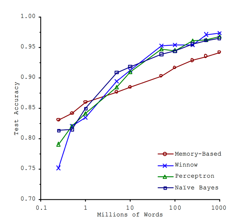
“Unreasonable Effectiveness”
- This must absolutely suck in practice, right?

From W06: Data Generating Process (DGP)
- You are a teacher trying to assess the causal impact of studying on homework scores
- Let \(S\) = hours of studying, \(H\) = homework score
- So far so good: we could estimate the relationship via (e.g.) regression
\[ h_i = \beta_0 + \beta_1 s_i + \varepsilon_i \]
My Dog Ate My Homework
- The issue: for some students \(h_i\) is missing, since their dog ate their homework
- Let \(D = \begin{cases}1 &\text{if dog ate homework} \\ 0 &\text{otherwise}\end{cases}\)
- This means we don’t observe \(H\) but \(H^* = \begin{cases} H &\text{if }D = 0 \\ \texttt{NA} &\text{otherwise}\end{cases}\)
- In the easy case, let’s say that dogs eat homework at random (i.e., without reference to \(S\) or \(H\)). Then we say \(H\) is “missing at random”. Our PGM now looks like:
My Dog Ate My Homework Because of Reasons

There are scarier alternatives, though! What if…
Dogs eat homework because their owner studied so much that the dog got ignored?
Dogs hate sloppy work, and eat bad homework that would have gotten a low score
Noisy homes (\(Z = 1\)) cause dogs to get agitated and eat homework more often, and students do worse
Why Do We Need To Think About DGPs?
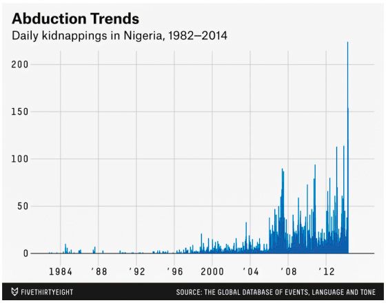
Presumed DGP:
Actual DGP:
Relevance to Clustering
- Let \(\boldsymbol\mu_1 = (0.2, 0.8)^\top\), \(\boldsymbol\mu_2 = (0.8, 0.2)^\top\), \(\Sigma = \text{diag}(1/64)\), and \(\mathbf{X} = (X_1, X_2)\).
- \(X_1 \sim \boldsymbol{\mathcal{N}}_2(\boldsymbol\mu_1, \Sigma)\), \(X_2 \sim \boldsymbol{\mathcal{N}}_2(\boldsymbol\mu_2, \Sigma)\)
Code
library(tidyverse)
library(ggforce)
library(MASS)
library(patchwork)
N <- 50
Mu1 <- c(0.2, 0.8)
Mu2 <- c(0.8, 0.2)
sigma <- 1/24
# Data for concentric circles
circle_df <- tribble(
  ~x0, ~y0, ~r, ~Cluster, ~whichR,
  Mu1[1], Mu1[2], sqrt(sigma), "C1", 1,
  Mu2[1], Mu2[2], sqrt(sigma), "C2", 1,
  Mu1[1], Mu1[2], 2 * sqrt(sigma), "C1", 2,
  Mu2[1], Mu2[2], 2 * sqrt(sigma), "C2", 2,
  Mu1[1], Mu1[2], 3 * sqrt(sigma), "C1", 3,
  Mu2[1], Mu2[2], 3 * sqrt(sigma), "C2", 3
)
#print(circle_df)
Sigma <- matrix(c(sigma,0,0,sigma), nrow=2)
#print(Sigma)
x1_df <- as_tibble(mvrnorm(N, Mu1, Sigma))
x1_df <- x1_df |> mutate(
  Cluster='C1'
)
x2_df <- as_tibble(mvrnorm(N, Mu2, Sigma))
x2_df <- x2_df |> mutate(
  Cluster='C2'
)
cluster_df <- bind_rows(x1_df, x2_df)
cluster_df <- cluster_df |> rename(
  x=V1, y=V2
)
known_plot <- ggplot(cluster_df) +
  geom_point(
    data = circle_df,
    aes(x=x0, y=y0)
  ) +
  geom_circle(
    data = circle_df,
    aes(x0=x0, y0=y0, r=r, fill=Cluster),
    linewidth = g_linewidth,
    alpha = 0.25
  ) +
  geom_point(
    data=cluster_df,
    aes(x=x, y=y, fill=Cluster),
    size = g_pointsize / 2,
    shape = 21
  ) +
  dsan_theme("full") +
  coord_fixed() +
  labs(
    x = "x",
    y = "y",
    title = "Data with Known Clusters"
  ) +
  scale_fill_manual(values=c(cbPalette[2], cbPalette[1], cbPalette[3], cbPalette[4])) +
  scale_color_manual(values=c(cbPalette[1], cbPalette[2], cbPalette[3], cbPalette[4]))
unknown_plot <- ggplot(cluster_df) +
  geom_point(
    data=cluster_df,
    aes(x=x, y=y),
    size = g_pointsize / 2,
    #shape = 21
  ) +
  dsan_theme("full") +
  coord_fixed() +
  labs(
    x = "x",
    y = "y",
    title = "Same Data with Unknown Clusters"
  )
cluster_df |> write_csv("assets/cluster_data.csv")
known_plot + unknown_plot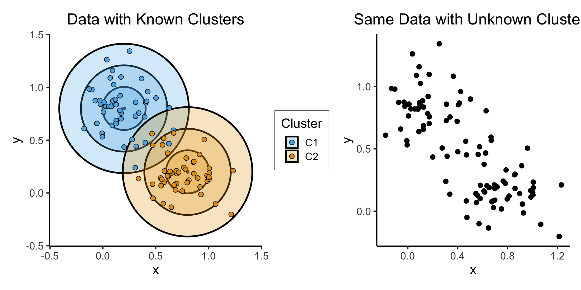
Clusters as Latent Variables
- Recall the Hidden Markov Model (one of many examples):
Modeling the Latent Distribution
- This observed/latent distinction gives us a modeling framework for inferring “underlying” distributions from data!
- Let’s begin with an overly-simple model: only one cluster (all data drawn from a single normal distribution)
Probability that RV \(X_i\) takes on value \(\mathbf{v}\):
\[ \begin{align*} &\Pr(X_i = \mathbf{v} \mid \param{\boldsymbol\theta_\mathcal{D}}) = \varphi_2(\mathbf{v}; \param{\boldsymbol\mu}, \param{\mathbf{\Sigma}}) \end{align*} \]
where \(\varphi_2(\mathbf{v}; \boldsymbol\mu, \mathbf{\Sigma})\) is pdf of \(\boldsymbol{\mathcal{N}}_2(\boldsymbol\mu, \mathbf{\Sigma})\).
Let \(\mathbf{X} = (X_1, \ldots, X_N)\), \(\mathbf{V} = (\mathbf{v}_1, \ldots, \mathbf{v}_N)\)
Probability that RV \(\mathbf{X}\) takes on values \(\mathbf{V}\):
\[ \begin{align*} &\Pr(\mathbf{X} = \mathbf{V} \mid \param{\boldsymbol\theta_\mathcal{D}}) \\ &= \Pr(X_1 = \mathbf{v}_1 \mid \paramDist) \times \cdots \times \Pr(X_N = \mathbf{v}_N \mid \paramDist) \end{align*} \]
So How Do We Infer Latent Vars From Data?
If only we had some sort of method for estimating which values of our unknown parameters \(\paramDist\) are most likely to produce our observed data \(\mathbf{X}\)
![]()
The diagram on the previous slide gave us an equation
\[ \begin{align*} \Pr(\mathbf{X} = \mathbf{V} \mid \param{\boldsymbol\theta_\mathcal{D}}) = \Pr(X_1 = \mathbf{v}_1 \mid \paramDist) \times \cdots \times \Pr(X_N = \mathbf{v}_N \mid \paramDist) \end{align*} \]
And we know that, when we consider the data as given and view this probability as a function of the parameters, we write it as
\[ \begin{align*} \lik(\mathbf{X} = \mathbf{V} \mid \param{\boldsymbol\theta_\mathcal{D}}) = \lik(X_1 = \mathbf{v}_1 \mid \paramDist) \times \cdots \times \lik(X_N = \mathbf{v}_N \mid \paramDist) \end{align*} \]
We want to find the most likely \(\paramDist\), that is, \(\boldsymbol\theta^*_\mathcal{D} = \argmax_{\paramDist}\mathcal{L}(\mathbf{X} = \mathbf{V} \mid \paramDist)\)
This value \(\boldsymbol\theta^*_\mathcal{D}\) is called the Maximum Likelihood Estimate of \(\paramDist\), and is easy to find using calculus tricks1
Handling Multiple Clusters
Probability \(X_i\) takes on value \(\mathbf{v}\):
\[ \begin{align*} &\Pr(X_i = \mathbf{v} \mid \param{C_i} = c_i; \; \param{\boldsymbol\theta_\mathcal{D}}) \\ &= \begin{cases} \varphi_2(v; \param{\boldsymbol\mu_1}, \param{\mathbf{\Sigma}}) &\text{if }c_i = 1 \\ \varphi_2(v; \param{\boldsymbol\mu_2}, \param{\mathbf{\Sigma}}) &\text{otherwise,} \end{cases} \end{align*} \]
where \(\varphi_2(v; \boldsymbol\mu, \mathbf{\Sigma})\) is pdf of \(\boldsymbol{\mathcal{N}}_2(\boldsymbol\mu, \mathbf{\Sigma})\).
Let \(\mathbf{C} = (\underbrace{C_1}_{\text{RV}}, \ldots, C_N)\), \(\mathbf{c} = (\underbrace{c_1}_{\mathclap{\text{scalar}}}, \ldots, c_N)\)
- Probability that RV \(\mathbf{X}\) takes on values \(\mathbf{V}\):
\[ \begin{align*} &\Pr(\mathbf{X} = \mathbf{V} \mid \param{\mathbf{C}} = \mathbf{c}; \; \param{\boldsymbol\theta_\mathcal{D}}) \\ &= \Pr(X_1 = \mathbf{v}_1 \mid \param{C_1} = c_1; \; \paramDist) \times \cdots \times \Pr(X_N = \mathbf{v}_N \mid \param{C_N} = c_N; \; \paramDist) \end{align*} \]
- It’s the same math as before! Find \((\mathbf{C}^*, \boldsymbol\theta^*_\mathcal{D}) = \argmax_{\param{\mathbf{C}}, \, \paramDist}\mathcal{L}(\mathbf{X} = \mathbf{V} \mid \param{\mathbf{C}}; \; \param{\boldsymbol\theta_\mathcal{D}})\)
In Code!
Code
import pandas as pd
import numpy as np
import sklearn
sklearn.set_config(display = 'text')
from sklearn.mixture import GaussianMixture
cluster_df = pd.read_csv("assets/cluster_data.csv")
X = cluster_df[['x','y']].values
estimator = GaussianMixture(n_components=2, covariance_type="spherical", max_iter=20, random_state=5000);
estimator.fit(X);
y_pred = estimator.predict(X)
# Gather everything into a .csv
# The estimated means
mean_df = pd.DataFrame(estimator.means_).transpose()
mean_df.columns = ['x','y']
mean_df['Estimated Centroid'] = ['mu1','mu2']
mean_df['Estimated Cluster'] = ['E1', 'E2']
mean_df['Estimated Cluster Mapped'] = ['C1', 'C2']
cov_array = estimator.covariances_
sigma1 = np.sqrt(cov_array[0])
sigma2 = np.sqrt(cov_array[1])
mean_df['Estimated Sigma'] = [sigma1,sigma2]
mean_df['Estimated 2Sigma'] = [2*sigma1, 2*sigma2]
mean_df['Estimated 3Sigma'] = [3*sigma1, 3*sigma2]
mean_df.to_csv("assets/sklearn_mean_df.csv", index=False)
# The estimated covariance matrix
cov_df = pd.DataFrame({'c1': [1, cov_array[0]], 'c2': [cov_array[1], 1]})
cov_df.to_csv("assets/sklearn_cov_df.csv", index=False)
# And the predicted clusters
pred_df = pd.DataFrame({'Estimated Cluster': y_pred})
pred_df['Estimated Cluster'] = pred_df['Estimated Cluster'].apply(lambda x: 'E1' if x == 0 else 'E2')
pred_df['Estimated Cluster Mapped'] = pred_df['Estimated Cluster'].apply(lambda x: 'C1' if x == 'E1' else 'C2')
pred_df.to_csv("assets/sklearn_pred_df.csv", index=False)
Distribution Estimation Results
Code
# Data for concentric circles
mean_df <- read_csv("assets/sklearn_mean_df.csv")
#print(mean_df)
cov_df <- read_csv("assets/sklearn_cov_df.csv")
#print(cov_df)
pred_df <- read_csv("assets/sklearn_pred_df.csv")
# Merge the predicted clusters into cluster_df
cluster_df <- bind_cols(cluster_df, pred_df)
cluster_df <- cluster_df |> mutate(
  Correct = as.numeric(`Estimated Cluster Mapped` == Cluster)
)
correct_df <- cluster_df |> filter(Correct == 1)
incorrect_df <- cluster_df |> filter(Correct == 0)
#print(cluster_df)
# Keep only the 3*Sigma circle
# compare_circle_df <- circle_df |> filter(
#   whichR == 3
# )
#print(mean_df)
#print(compare_circle_df)
compare_plot <- ggplot(cluster_df) +
  geom_point(
    data = mean_df,
    aes(
      x=x, y=y,
      #fill=`Estimated Cluster`
    )
  ) +
  geom_point(
    data = circle_df,
    aes(
      x=x0, y=y0,
      #fill=Cluster
    )
  ) +
  geom_circle(
    data = mean_df,
    aes(
      x0=x, y0=y,
      r=`Estimated Sigma`,
      color=`Estimated Cluster`
      #fill=`Estimated Centroid`
    ),
    linewidth = g_linewidth,
    alpha = 0.25
  ) +
  geom_circle(
    data = mean_df,
    aes(
      x0=x, y0=y,
      r=`Estimated 2Sigma`,
      color=`Estimated Cluster`
      #fill=`Estimated Centroid`
    ),
    linewidth = g_linewidth,
    alpha = 0.25
  ) +
  geom_circle(
    data = mean_df,
    aes(
      x0=x, y0=y,
      r=`Estimated 3Sigma`,
      color=`Estimated Cluster`
      #fill=`Estimated Cluster`
    ),
    linewidth = g_linewidth,
    alpha = 0.25
  ) +
  geom_circle(
    data = circle_df,
    aes(
      x0=x0, y0=y0,
      r=r,
      color=Cluster
      #fill=Cluster
    ),
    linewidth = g_linewidth,
    alpha = 0.25
  ) +
  dsan_theme("full") +
  coord_fixed() +
  labs(
    x = "x",
    y = "y",
    title = "DGP vs. Estimated Clusters",
    fill = "MLE",
    color = "MLE",
    shape = "Correct?"
  ) +
  scale_shape_manual(values = c(4,21)) +
  scale_color_manual(values=c(cbPalette[2], cbPalette[1], cbPalette[3], cbPalette[4]))
compare_plot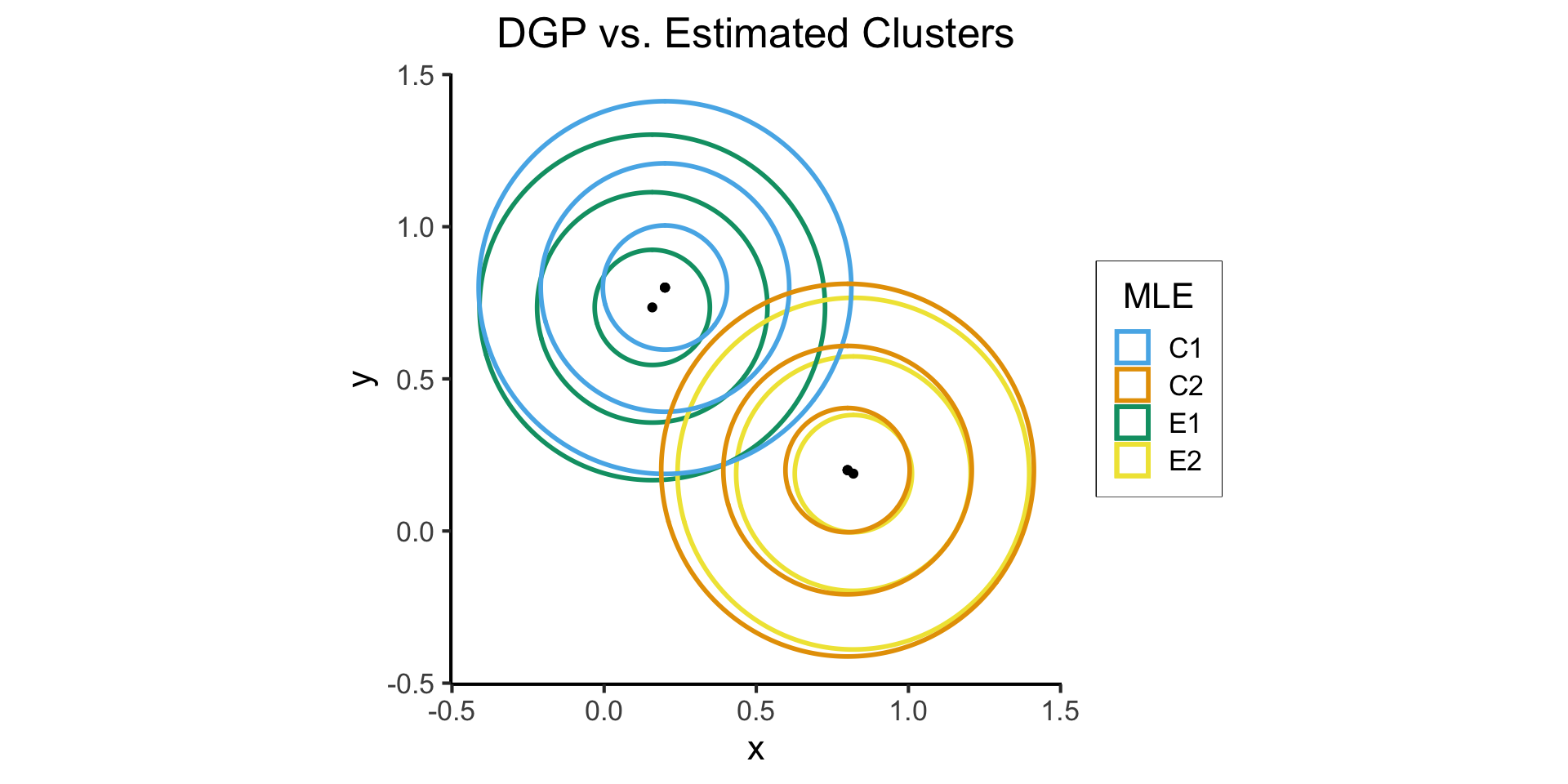
Clustering Results
Code
est_plot <- ggplot(cluster_df) +
  # geom_point(
  #   data = mean_df,
  #   aes(x=x, y=y)
  # ) +
  geom_circle(
    data = mean_df,
    aes(
      x0=x, y0=y,
      r=`Estimated Sigma`,
      fill=`Estimated Cluster Mapped`
    ),
    linewidth = g_linewidth,
    alpha = 0.25
  ) +
  geom_circle(
    data = mean_df,
    aes(x0=x, y0=y, r=`Estimated 2Sigma`, fill=`Estimated Cluster Mapped`),
    linewidth = g_linewidth,
    alpha = 0.25
  ) +
  geom_circle(
    data = mean_df,
    aes(x0=x, y0=y, r=`Estimated 3Sigma`, fill=`Estimated Cluster Mapped`),
    linewidth = g_linewidth,
    alpha = 0.25
  ) +
  geom_point(
    data=cluster_df,
    aes(
      x=x, y=y,
      fill=factor(`Estimated Cluster Mapped`),
      shape=factor(Correct)
    ),
    size = g_pointsize / 2,
    stroke = 0.75
  ) +
  geom_point(
    data=incorrect_df,
    aes(x=x, y=y),
    color='black',
    shape = 4,
    size = g_pointsize / 2,
    stroke = 2
  ) +
  geom_point(
    data=incorrect_df,
    aes(x=x, y=y),
    color=cbPalette[4],
    shape = 4,
    size = g_pointsize / 2,
    stroke = 0.8
  ) +
  dsan_theme("full") +
  coord_fixed() +
  labs(
    x = "x",
    y = "y",
    title = "Data with Estimated Clusters",
    fill = "MLE",
    color = "MLE",
    shape = "Correct?"
  ) +
  scale_shape_manual(values = c(4,21)) +
  scale_fill_manual(values=c(cbPalette[3], cbPalette[4])) +
  scale_color_manual(values=c(cbPalette[3], cbPalette[4]))
known_plot + est_plot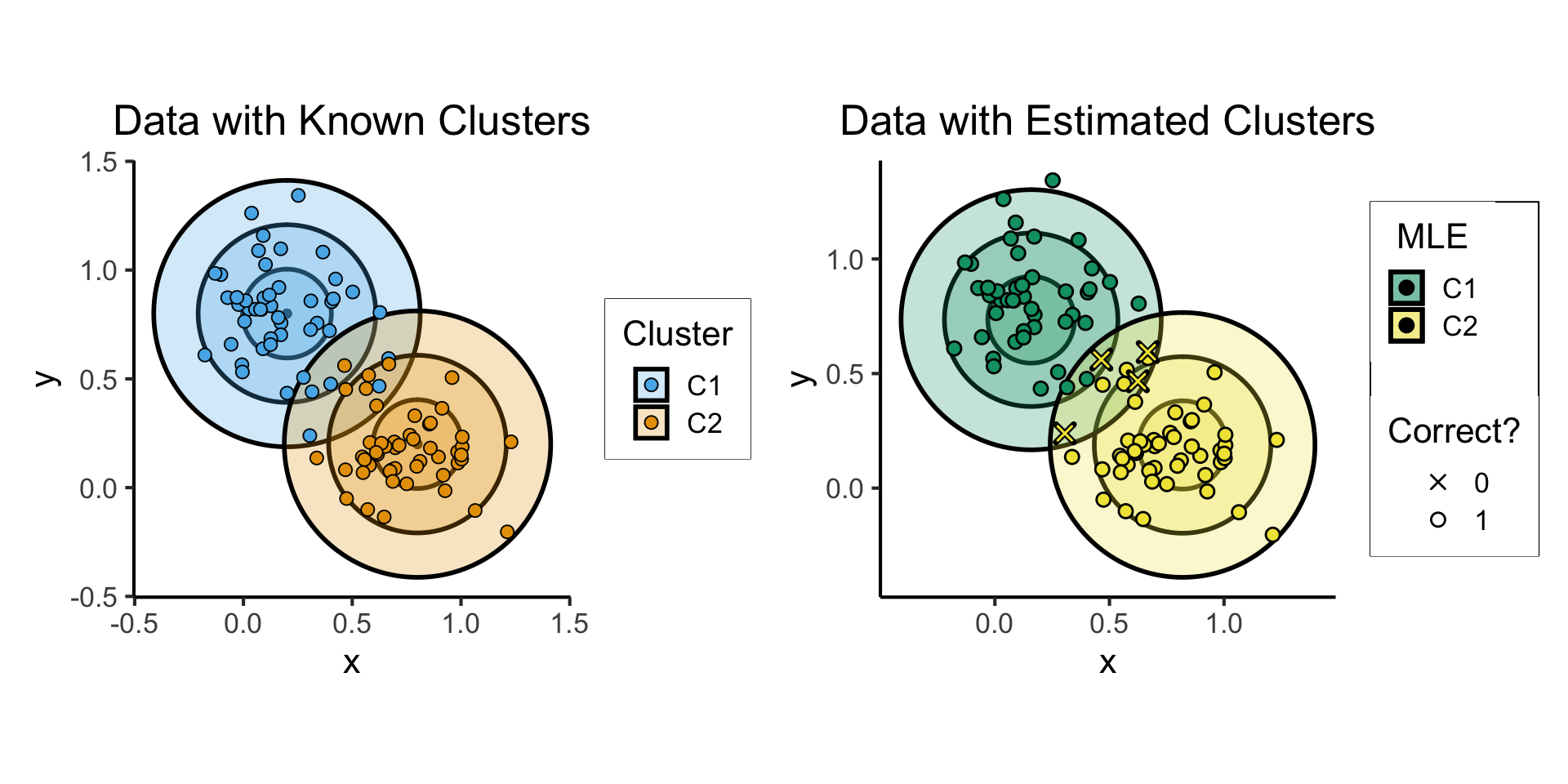
Clustering In General
- What makes a “good” cluster?
- In previous example, “good” meant that it recovered our DGP
- In an EDA context, we may not have a well-formulated DGP in mind…
Unsupervised Clustering: Heuristics
| Heuristic 1 | Heuristic 2 |
|---|---|
| Points in same cluster should be similar | Points in different clusters should be dissimilar |
You could take these two heuristics, formalize them, and derive the rest of lecture 😉
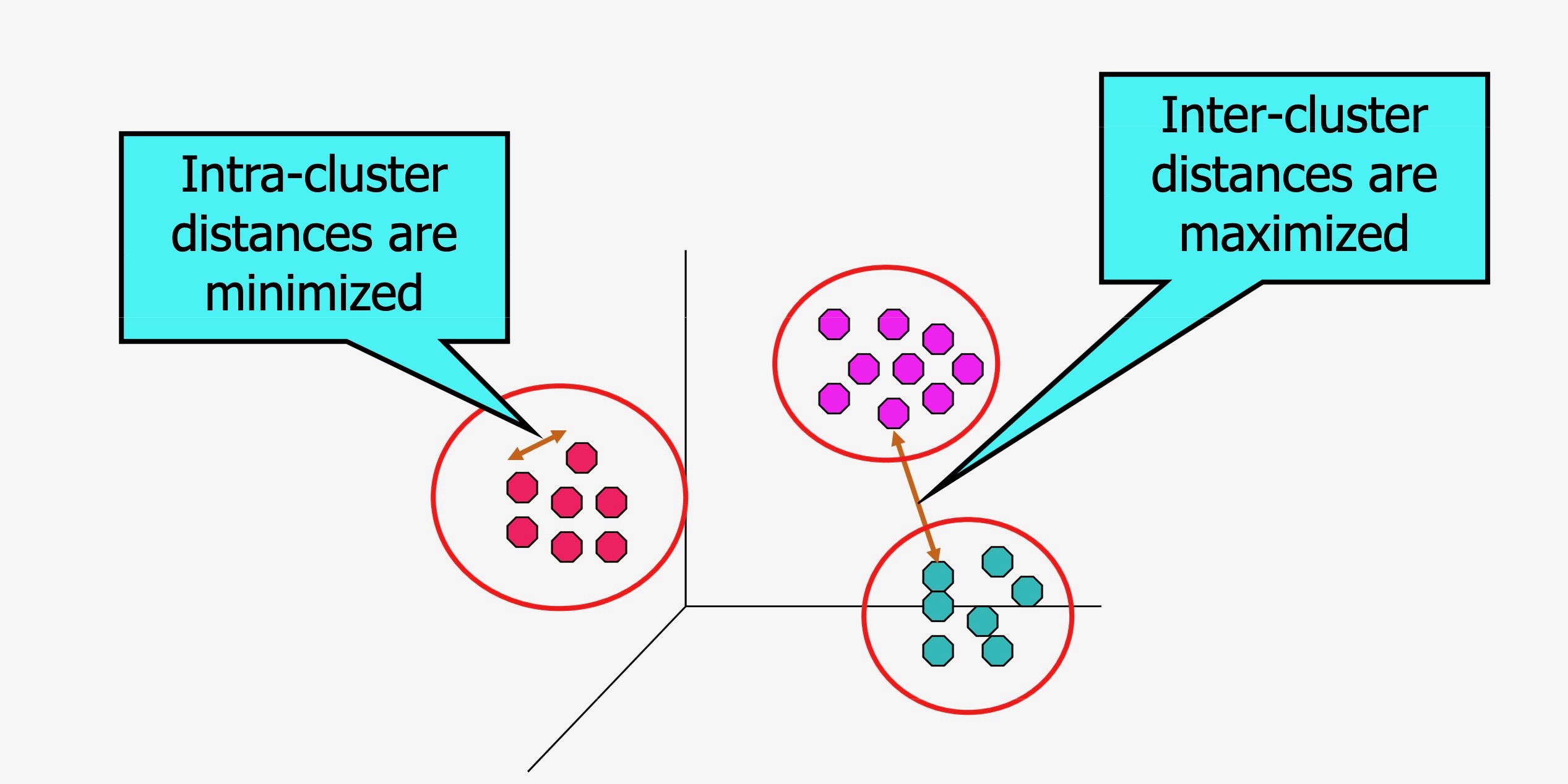
Image from Introduction to Machine Learning, University of Washington (2012)
Hierarchical Clustering
- If our task is to partition, we’re done!
- If our task is to infer a hierarchy, we can also think about a spectrum of coarse-grained to fine-grained clusterings:
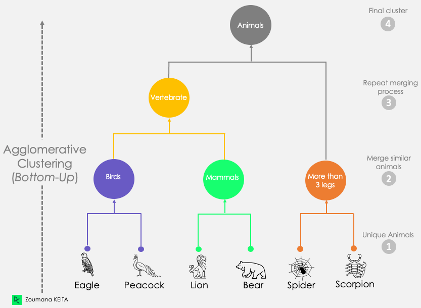
Hierarchical Clustering \(\rightarrow\) Multilevel Modeling
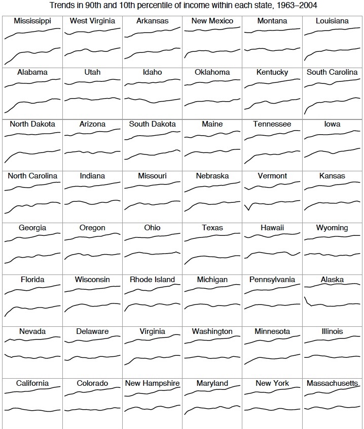
- Extremely powerful modeling tool for statistical inference!
- Learning about eagles \(\implies\) learning about birds
- Surveying DSAN 5000 students \(\implies\) Georgetown students
- We can pool information from US states into national estimates
- And, when we compute averages, we can take into account our relative certainty/uncertainty about units at each level (read more here)
Image from Gelman (2009)
In Practice
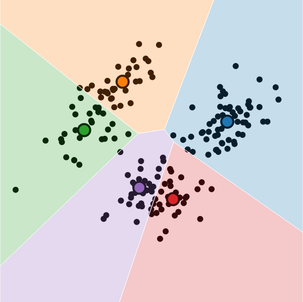
K-Means Clustering
What is K-Means Clustering?
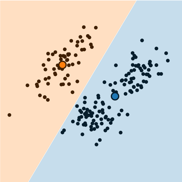
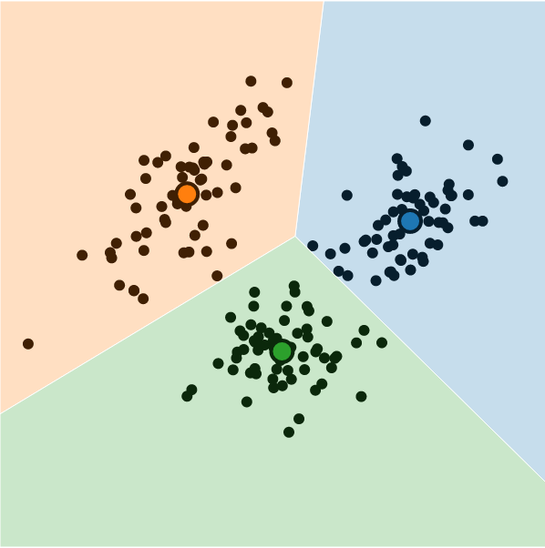
- Operationalizes our two heuristics by simultaneously:
- Maximizing within-cluster similarity
- Minimizing between-cluster similarity
K-Means Clustering Algorithm
- Data \(\mathbf{X} = (X_1 = \mathbf{x}_1, \ldots, X_N = \mathbf{x}_N)\)
- Distance metric \(d(\mathbf{v}_1, \mathbf{v}_2)\)
- Hyperparameter value for \(K\) (⁉️)
- Assign each point \(\mathbf{x}_i\) to a cluster \(C_i \in \{1, \ldots, K\}\) (so \(S_j = \{\mathbf{x}_i \mid C_i = j\}\) is the set of points assigned to cluster \(j\))
K-Means Clustering Algorithm
Initialize \(K\) random centroids \(\boldsymbol\mu_1, \ldots, \boldsymbol\mu_K\)
(Re-)Compute distance \(d(\mathbf{x}_i, \boldsymbol\mu_j)\) from each point \(\mathbf{x}_i\) to each centroid \(\boldsymbol\mu_j\)
(Re-)Assign points to class of nearest centroid: \(C_i = \argmin_j d(\mathbf{x}_i, \boldsymbol\mu_j)\)
(Re-)compute centroids as mean of points in each cluster:
\[ \mu_j^\text{new} \leftarrow \frac{1}{|S_j|}\sum_{\mathbf{x}_i \in S_j}\mathbf{x}_i \]
Repeat Steps 2-4 until convergence
In Pictures
In Code + Pictures
Code
import pandas as pd
import matplotlib.colors
from sklearn.cluster import KMeans
cluster_df = pd.read_csv("assets/cluster_data.csv")
X = cluster_df[['x','y']].values
kmc_model = KMeans(
  n_clusters=2,
  init='k-means++',
  verbose=0,
  random_state=5000,
  copy_x=True,
  algorithm='lloyd'
);
kmc_model.fit(X);
y_pred_vals = kmc_model.predict(X)
y_pred_df = pd.DataFrame({'y_pred': y_pred_vals})
y_pred_df.to_csv("assets/kmc_preds.csv", index=False)
kmc_centroid_df = pd.DataFrame(kmc_model.cluster_centers_.transpose(), columns=['x','y'])
#disp(kmc_centroid_df)
kmc_centroid_df.to_csv("assets/kmc_centroids.csv", index=False)

import matplotlib.pyplot as plt
# Step size of the mesh. Decrease to increase the quality of the VQ.
h = 0.01  # point in the mesh [x_min, x_max]x[y_min, y_max].

# Plot the decision boundary. For that, we will assign a color to each
bpad = 0.05
x_min, x_max = X[:, 0].min() - bpad, X[:, 0].max() + bpad
y_min, y_max = X[:, 1].min() - bpad, X[:, 1].max() + bpad
xx, yy = np.meshgrid(np.arange(x_min, x_max, h), np.arange(y_min, y_max, h))

# Obtain labels for each point in mesh. Use last trained model.
Z = kmc_model.predict(np.c_[xx.ravel(), yy.ravel()])

# Put the result into a color plot
#custom_cmap = matplotlib.colors.LinearSegmentedColormap.from_list("", ["red","violet","blue"])
#custom_cmap = matplotlib.colors.ListedColormap(['white', 'red'])
#custom_cmap = matplotlib.colors.ListedColormap(cb_palette).reversed()
custom_cmap = matplotlib.colors.ListedColormap([cb_palette[0], cb_palette[2], cb_palette[1]])
Z = Z.reshape(xx.shape)
plt.figure(1)
plt.clf()
plt.imshow(
    Z,
    interpolation="nearest",
    extent=(xx.min(), xx.max(), yy.min(), yy.max()),
    #cmap=plt.cm.Paired,
    cmap=custom_cmap,
    aspect="auto",
    origin="lower",
)

# And plot the points
plt.plot(X[:, 0], X[:, 1], "o", markersize=6, color='white', markerfacecolor='black', alpha=0.75)
# Plot the centroids as a white X
centroids = kmc_model.cluster_centers_
plt.scatter(
    centroids[:, 0],
    centroids[:, 1],
    marker="*",
    s=250,
    linewidths=1.5,
    color='white',
    facecolor='black',
    zorder=10,
)
# Plot gaussian means as... smth else
plt.scatter(
    [0.2,0.8],
    [0.8,0.2],
    marker="*",
    s=250,
    linewidths=1.5,
    color=cb_palette[3],
    facecolor='black',
    zorder=9,
)
plt.title(
    "K-means clustering on the Gaussian mixture data"
)
plt.legend([
  'Original Data',
  'K-Means Centroids',
  'True Centroids (DGP)'
])
plt.show()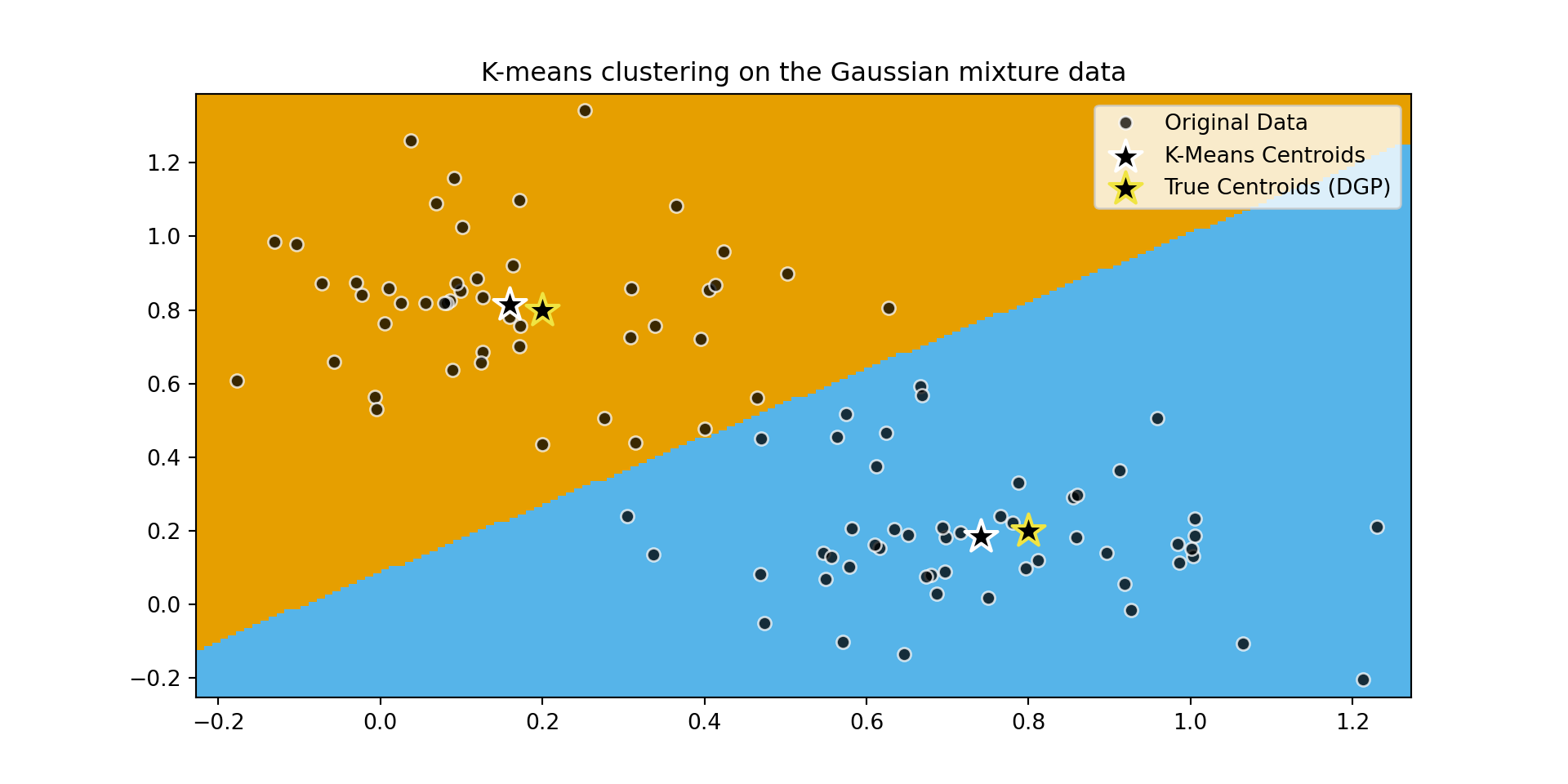
Adapted from Scikit-learn User Guide
DBSCAN
Code
import time
import warnings
from itertools import cycle, islice

import matplotlib.pyplot as plt
import numpy as np

from sklearn import cluster, datasets, mixture
from sklearn.neighbors import kneighbors_graph
from sklearn.preprocessing import StandardScaler

# ============
# Generate datasets. We choose the size big enough to see the scalability
# of the algorithms, but not too big to avoid too long running times
# ============
n_samples = 500
seed = 30
noisy_circles = datasets.make_circles(
    n_samples=n_samples, factor=0.5, noise=0.05, random_state=seed
)
noisy_moons = datasets.make_moons(n_samples=n_samples, noise=0.05, random_state=seed)
blobs = datasets.make_blobs(n_samples=n_samples, random_state=seed)
rng = np.random.RandomState(seed)
no_structure = rng.rand(n_samples, 2), None

# Anisotropicly distributed data
random_state = 170
X, y = datasets.make_blobs(n_samples=n_samples, random_state=random_state)
transformation = [[0.6, -0.6], [-0.4, 0.8]]
X_aniso = np.dot(X, transformation)
aniso = (X_aniso, y)

# blobs with varied variances
varied = datasets.make_blobs(
    n_samples=n_samples, cluster_std=[1.0, 2.5, 0.5], random_state=random_state
)

# ============
# Set up cluster parameters
# ============
plt.figure(figsize=(9 * 2 + 3, 13))
plt.subplots_adjust(
    left=0.02, right=0.98, bottom=0.001, top=0.95, wspace=0.05, hspace=0.01
)

plot_num = 1

default_base = {
    "quantile": 0.3,
    "eps": 0.3,
    "damping": 0.9,
    "preference": -200,
    "n_neighbors": 3,
    "n_clusters": 3,
    "min_samples": 7,
    "xi": 0.05,
    "min_cluster_size": 0.1,
    "allow_single_cluster": True,
    "hdbscan_min_cluster_size": 15,
    "hdbscan_min_samples": 3,
    "random_state": 42,
}

datasets = [
    (
        noisy_circles,
        {
            "damping": 0.77,
            "preference": -240,
            "quantile": 0.2,
            "n_clusters": 2,
            "min_samples": 7,
            "xi": 0.08,
        },
    ),
    (
        noisy_moons,
        {
            "damping": 0.75,
            "preference": -220,
            "n_clusters": 2,
            "min_samples": 7,
            "xi": 0.1,
        },
    ),
    # (
    #     varied,
    #     {
    #         "eps": 0.18,
    #         "n_neighbors": 2,
    #         "min_samples": 7,
    #         "xi": 0.01,
    #         "min_cluster_size": 0.2,
    #     },
    # ),
    (
        aniso,
        {
            "eps": 0.15,
            "n_neighbors": 2,
            "min_samples": 7,
            "xi": 0.1,
            "min_cluster_size": 0.2,
        },
    ),
    (blobs, {"min_samples": 7, "xi": 0.1, "min_cluster_size": 0.2}),
    (no_structure, {}),
]

for i_dataset, (dataset, algo_params) in enumerate(datasets):
    # update parameters with dataset-specific values
    params = default_base.copy()
    params.update(algo_params)

    X, y = dataset

    # normalize dataset for easier parameter selection
    X = StandardScaler().fit_transform(X)

    # estimate bandwidth for mean shift
    bandwidth = cluster.estimate_bandwidth(X, quantile=params["quantile"])

    # connectivity matrix for structured Ward
    connectivity = kneighbors_graph(
        X, n_neighbors=params["n_neighbors"], include_self=False
    )
    # make connectivity symmetric
    connectivity = 0.5 * (connectivity + connectivity.T)

    # ============
    # Create cluster objects
    # ============
    two_means = cluster.MiniBatchKMeans(
        n_clusters=params["n_clusters"],
        n_init="auto",
        random_state=params["random_state"],
    )
    ms = cluster.MeanShift(bandwidth=bandwidth, bin_seeding=True)
    # spectral = cluster.SpectralClustering(
    #     n_clusters=params["n_clusters"],
    #     eigen_solver="arpack",
    #     affinity="nearest_neighbors",
    #     random_state=params["random_state"],
    # )
    dbscan = cluster.DBSCAN(eps=params["eps"])
    average_linkage = cluster.AgglomerativeClustering(
        linkage="average",
        metric="cityblock",
        n_clusters=params["n_clusters"],
        connectivity=connectivity,
    )
    birch = cluster.Birch(n_clusters=params["n_clusters"])
    gmm = mixture.GaussianMixture(
        n_components=params["n_clusters"],
        covariance_type="full",
        random_state=params["random_state"],
    )

    clustering_algorithms = (
        ("MiniBatch\nKMeans", two_means),
        #("Affinity\nPropagation", affinity_propagation),
        ("MeanShift", ms),
        #("Spectral\nClustering", spectral),
        #("Ward", ward),
        ("Agglomerative\nClustering", average_linkage),
        ("DBSCAN", dbscan),
        #("HDBSCAN", hdbscan),
        #("OPTICS", optics),
        ("BIRCH", birch),
        ("Gaussian\nMixture", gmm),
    )

    for name, algorithm in clustering_algorithms:
        t0 = time.time()

        # catch warnings related to kneighbors_graph
        with warnings.catch_warnings():
            warnings.filterwarnings(
                "ignore",
                message="the number of connected components of the "
                + "connectivity matrix is [0-9]{1,2}"
                + " > 1. Completing it to avoid stopping the tree early.",
                category=UserWarning,
            )
            warnings.filterwarnings(
                "ignore",
                message="Graph is not fully connected, spectral embedding"
                + " may not work as expected.",
                category=UserWarning,
            )
            algorithm.fit(X)

        t1 = time.time()
        if hasattr(algorithm, "labels_"):
            y_pred = algorithm.labels_.astype(int)
        else:
            y_pred = algorithm.predict(X)

        plt.subplot(len(datasets), len(clustering_algorithms), plot_num)
        if i_dataset == 0:
            plt.title(name, size=18)

        colors = np.array(
            list(
                islice(
                    cycle(
                        [
                            "#377eb8",
                            "#ff7f00",
                            "#4daf4a",
                            "#f781bf",
                            "#a65628",
                            "#984ea3",
                            "#999999",
                            "#e41a1c",
                            "#dede00",
                        ]
                    ),
                    int(max(y_pred) + 1),
                )
            )
        )
        # add black color for outliers (if any)
        colors = np.append(colors, ["#000000"])
        plt.scatter(X[:, 0], X[:, 1], s=10, color=colors[y_pred])

        plt.xlim(-2.5, 2.5)
        plt.ylim(-2.5, 2.5)
        plt.xticks(())
        plt.yticks(())
        plt.text(
            0.99,
            0.01,
            ("%.2fs" % (t1 - t0)).lstrip("0"),
            transform=plt.gca().transAxes,
            size=15,
            horizontalalignment="right",
        )
        plot_num += 1

plt.show()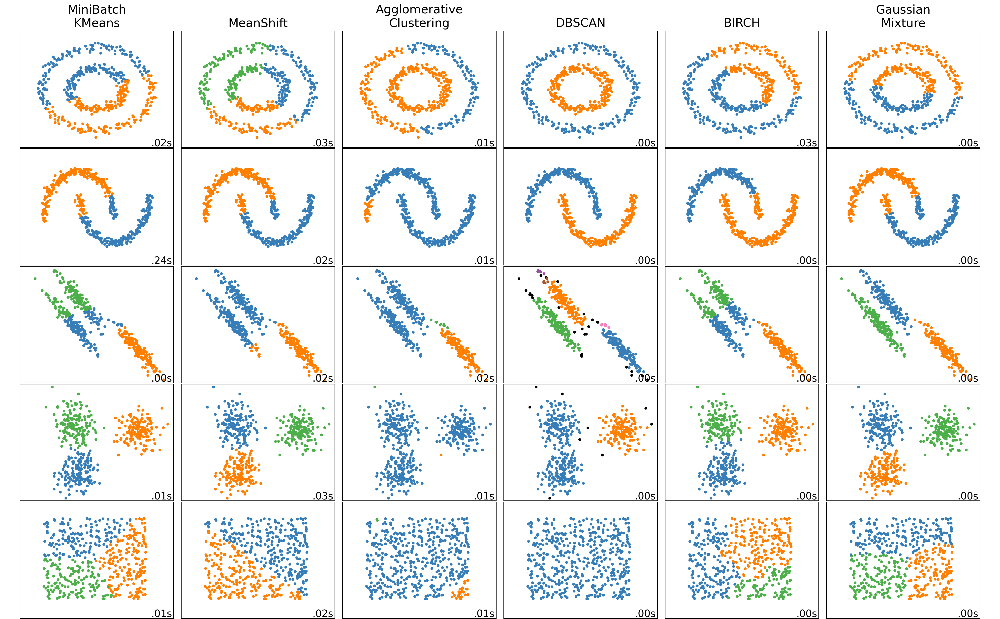
Adapted from Scikit-learn User Guide
Hyperparameter Tuning: More Heuristics
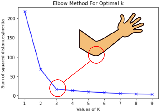
- Inertia: A measure of how “well-clustered” a dataset is
- Sum of squared distances of samples to their closest cluster center
- A good model is one with low inertia and low \(K\) (tradeoff, akin to bias-variance)
- Elbow Method: Find the \(K\) value after which decrease in inertia begins to slow →
References
DSAN 5000 W08: Supervised and Unsupervised Learning
