Week 6: Spatial Joins and Areal Weighted Interpolation

PPOL 6805 / DSAN 6750: GIS for Spatial Data Science
Fall 2026

Jeff Jacobs

jj1088@georgetown.edu

Wednesday, September 30, 2026

Doing Things with DE-9IM (Back to Binary Operations)

Slowing Down: 9IM (no DE yet!)

9IM Interior Boundary Exterior
Interior


Boundary


Exterior


Table 1: From OSGeo Project

Dimensionally Extended (DE) 9IM

9IM Interior Boundary Exterior
Interior
2

1

2
Boundary
1

0

1
Exterior
2

1

2
Table 2: From OSGeo Project

Crunching it Down into a Tiny Box

DE-9IM Interior Boundary Exterior
Interior 2 1 2
Boundary 1 0 1
Exterior 2 1 2

…And Then into a Tiny String

212101212

…And Then into an Infinitesimally-Small Point

DE-9IM Masks

  • Now terms can be given unambiguous, precise meaning!
st_overlaps() Interior Boundary Exterior
Interior T * T
Boundary * * *
Exterior T * *
  • Special Values (besides 0, 1, 2):
    • T: “True” (non-empty, st_dimension() >= 0)
    • F: “False” (empty, st_dimension() == NA)
    • *: “Wildcard” (Don’t care what the value is)
  • st_overlaps(): T*T***T**, st_equals(): T*F**FFF*

DE-9IM vs. Everyday Language

  • DE-9IM can (in theory) represent \(6^9 = 10~077~696\) possible geometric relationships!
  • The English language has like 10, and they’re ambiguous ☠️ (Compromise employed by GIS systems: allow multiple masks for same English word):
English Mask 212101212 Result
“Disjoint” FF*FF**** FALSE x not disjoint from y
“Touches” FT******* FALSE x doesn’t touch y
“Touches” F***T**** FALSE x doesn’t touch y
“Crosses” T*T***T** TRUE x crosses y
“Within” TF*F***** FALSE x is not within y
“Overlaps” T*T***T** TRUE x overlaps y

st_relate(): The Ultimate Predicate

Code
us_sf <- ne_states(iso_a2 = "US") |> add_colonies()
dc_sf <- us_sf |> filter(iso_3166_2 == "US-DC")
us_sf <- us_sf |> mutate(
    de9im = st_relate(us_sf, dc_sf),
    touches_dc = st_touches(us_sf, dc_sf, sparse = F)
  ) |>
  select(iso_3166_2, name, de9im, touches_dc) |>
  arrange(name)
us_sf

(If You Don’t Want to Scroll)

Code
us_sf |> filter(touches_dc)

Spatial Joins

Spatial Filter: Almost a Spatial Join

Code
set.seed(6805)
N <- 10
africa_sf <- ne_countries(continent = "Africa", scale = 50) |> select(geounit, gdp_md)
africa_union_sf <- sf::st_union(africa_sf)
africa_map <- mapview(africa_sf, label="geounit", legend=FALSE, col.regions=cb_palette[2], alpha.regions=0.5)
sampled_points_sf <- sf::st_sample(africa_union_sf, N) |> sf::st_sf() |> mutate(temp_c = runif(N, 0, 100), pop=rdunif(N, 1, 1000))
sampled_points_map <- mapview(sampled_points_sf, label="Random Point", col.regions=cb_palette[1], legend=FALSE)
countries_points_sf <- africa_sf[sampled_points_sf,]
filtered_map <- mapview(countries_points_sf, label="geounit", legend=FALSE, col.regions=cb_palette[2], alpha.regions=0.5)
(africa_map + sampled_points_map) | (filtered_map + sampled_points_map)

Spatial Filter \(\neq\) Spatial Join

  • Initial problem: Attributes of POINTs are not merged into attributes of POLYGONs
  • Deeper problem: How to merge multiple POINT attributes into single row?
POLYGON Attributes

\(\overset{?}{\leftarrow}\)

POINT Attributes
Code
countries_points_sf |> relocate(geometry, geounit)
Code
st_geometry(sampled_points_sf) <- c("geometry")
sampled_points_sf

Our First Real Spatial Join: st_join()

Code
joined_sf <- countries_points_sf |> st_join(sampled_points_sf)
joined_sf |> relocate(geounit, temp_c, pop) |> head()

But… We Were Still in Easy Mode

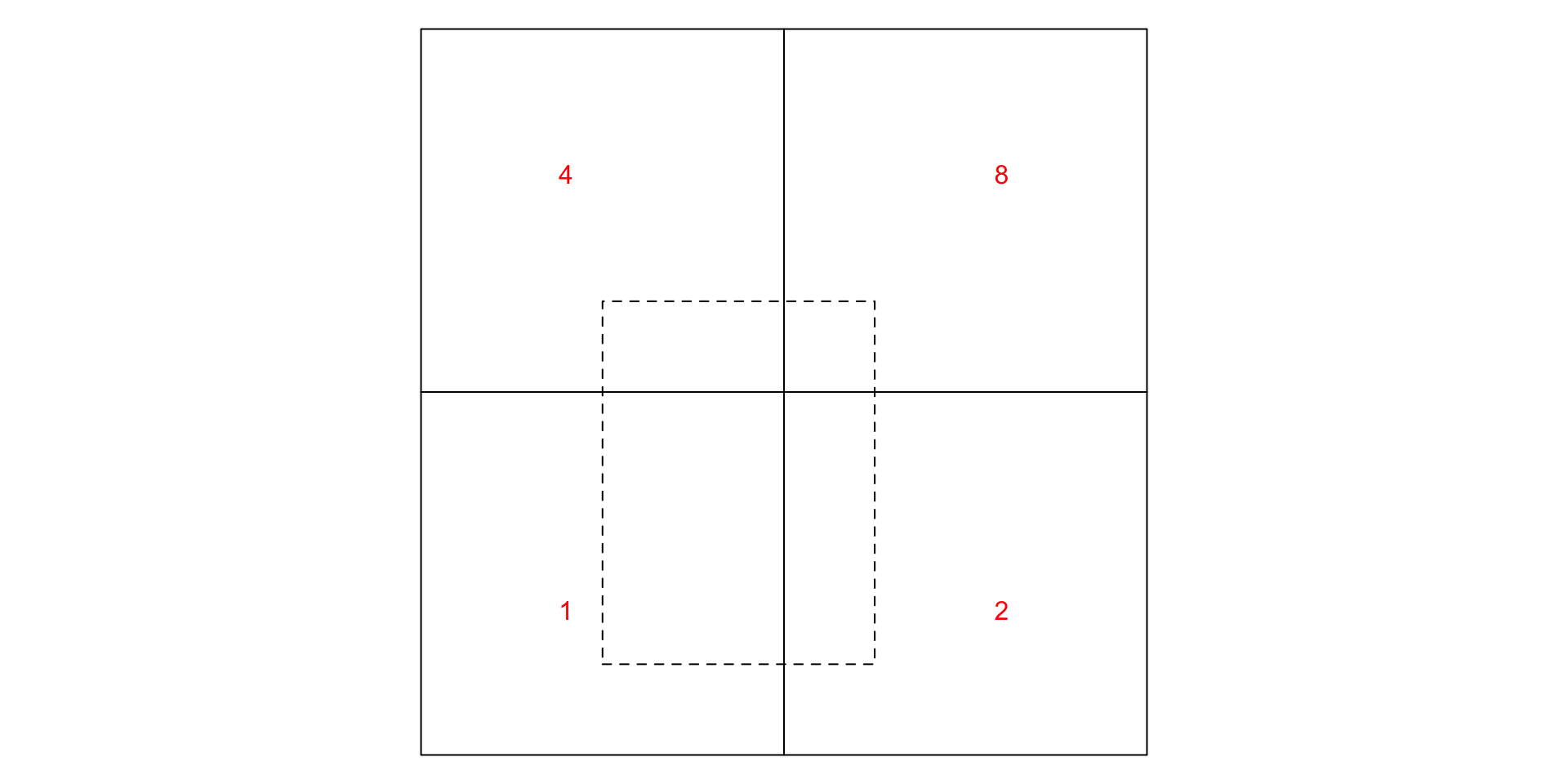
Every point could be matched to one country. But what if… 😱
Code
g <- st_make_grid(st_bbox(st_as_sfc("LINESTRING(0 0,1 1)")), n = c(2,2))
par(mar = rep(0,4))
plot(g)
plot(g[1] * diag(c(3/4, 1)) + c(0.25, 0.125), add = TRUE, lty = 2)
text(c(.2, .8, .2, .8), c(.2, .2, .8, .8), c(1,2,4,8), col = 'red')

Areal Weighted Interpolation

ZIP Codes vs. Census Tracts

Geographic Unit Administered By For
Census Tracts US Census Bureau Demographic statistics
We are in GeoID \(\overbrace{\underbrace{\large\texttt{11}}_{\small\text{State}}\underbrace{\large\texttt{001}}_{\small\text{County}}}^{\small\text{FIPS Code}}\overbrace{\underbrace{\large\texttt{0002}}_{\small\text{Number}}\underbrace{\large\texttt{01}}_{\small\text{Suffix}}}^{\small\text{Census Tract}}\): DC Census Tract 2.02
ZIP Code™ US Postal Service Mail delivery
We are in 20007 (20057 = Hilltop Campus West of 37th St NW!)
Topographic Quadrangles US Geological Survey Land resource management
We are in Washington West Quadrangle

ZIP Code Not On Geographic Spine!

Code
(dc_zip_df <- read_csv("dc.csv") |> arrange(desc(overlap)) |> mutate(geoid=format(geoid,scientific=F)))
Code
dc_zip_df |> select(overlap) |> sum() |> round(digits=3)
[1] 1

Spatially Intensive vs. Spatially Extensive

  • Extensive attributes: associated with a physical size (length, area, volume, counts of items). Ex: population count.
    • Associated with an area \(\implies\) if that area is cut into smaller areas, the population count needs to be split too
    • Constraint: The sum of the population counts for the smaller areas needs to equal the total population across the combined area
  • Intensive attributes: Not proportional to support: if the area is split, values may vary but on average remain the same. Ex: population density
    • If an area is split into smaller areas, population density is not split similarly!
    • The sum of population densities for the smaller areas is a meaningless measure
    • Constraint: the mean of the population density for the smaller areas needs to equal the overall population density across the combined area

Handling the Extensive Case

  • Assume the extensive attribute \(Y\) is uniformly distributed over a space \(S_i\) (e.g., for population counts we assume everyone is evenly-spaced across the region)

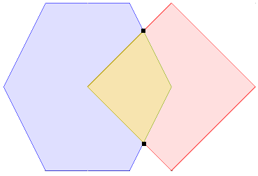
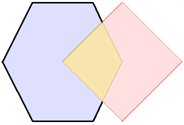
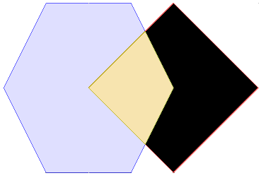
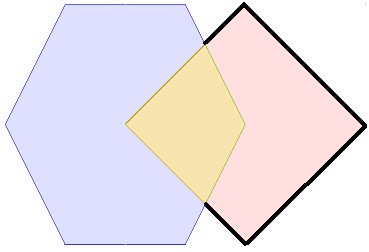
  • We first compute \(Y_{ij}\), derived from \(Y_i\) for a sub-area of \(S_i\), \(A_{ij} = S_i \cap T_j\):

    \[ \hat{Y}_{ij}(A_{ij}) = \frac{|A_{ij}|}{|S_i|}Y_i(S_i) \]

    where \(|\cdot|\) denotes area.

  • Then we can compute \(Y_j(T_j)\) by summing all the elements over area \(T_j\):

\[ \hat{Y}_j(T_j) = \sum_{i=1}^{p}\frac{|A_{ij}|}{|S_i|}Y_i(S_i) \]

Handling the Intensive Case

  • Assume the variable \(Y\) has constant value over a space \(S_i\) (e.g., population density in assumed to be the same across all sub-areas)
  • Then the estimate for a sub-area is the same as the estimate for the total area:

\[ \hat{Y}_{ij} = Y_i(S_i) \]

  • So that we can obtain estimates of \(Y\) for new spatial units \(T_j\) via area-weighted average of the source values:

\[ \hat{Y}_j(T_j) = \sum_{i=1}^{p}\frac{|A_{ij}|}{|T_j|}Y_j(S_i) \]

Let’s Go See It In Action!


Week 6 Lab: Interpolating Kurdistan

References