Week 3: Unary Operations

PPOL 6805 / DSAN 6750: GIS for Spatial Data Science
Fall 2024

Jeff Jacobs

jj1088@georgetown.edu

Wednesday, September 11, 2024

How to Do Things with Geometries

From the sf Cheatsheet

HW1 \(\rightarrow\) HW2

• Congrats on finishing HW1! You now know how to create geometries with sf and terra
• So now, what can you do with them?
• For example, we’d like to be able to say things like:
  • “The new lamppost cannot be placed at \((x, y)\), since there is already a building there!”
  • “There are \(N_1\) lampposts in County 1, and \(N_2\) lampposts in County 2”
  • “The average resident in Neighborhood A lives 2 km away from their nearest bus stop

First Things First: Loading and Saving

• Note how there were no data files in HW1 😱
• From HW2 onwards (and in your GIS life), we’ll:
  • Download from e.g. city Open Data Portals: geo data files, but also loading on-the-fly (this week)
  • Summarize/aggregate (this week and next week)
  • Visualize findings (“Mapping Libraries” unit)

Vector Formats

Shapefiles (.shp et al.)

A shape“file” is actually (at least) three separate files bundled together:

• Mandatory .shp: Containing feature geometries
• Mandatory .shx: Positional indices
• Mandatory .dbf: Data attributes
• Optional .prj: Coordinate reference system
• Optional .xml: Metadata

Shapefiles

Let’s see what’s inside the shapefile we first saw in Week 1, containing data on DC’s Census Tracts: Census Tracts in 2020

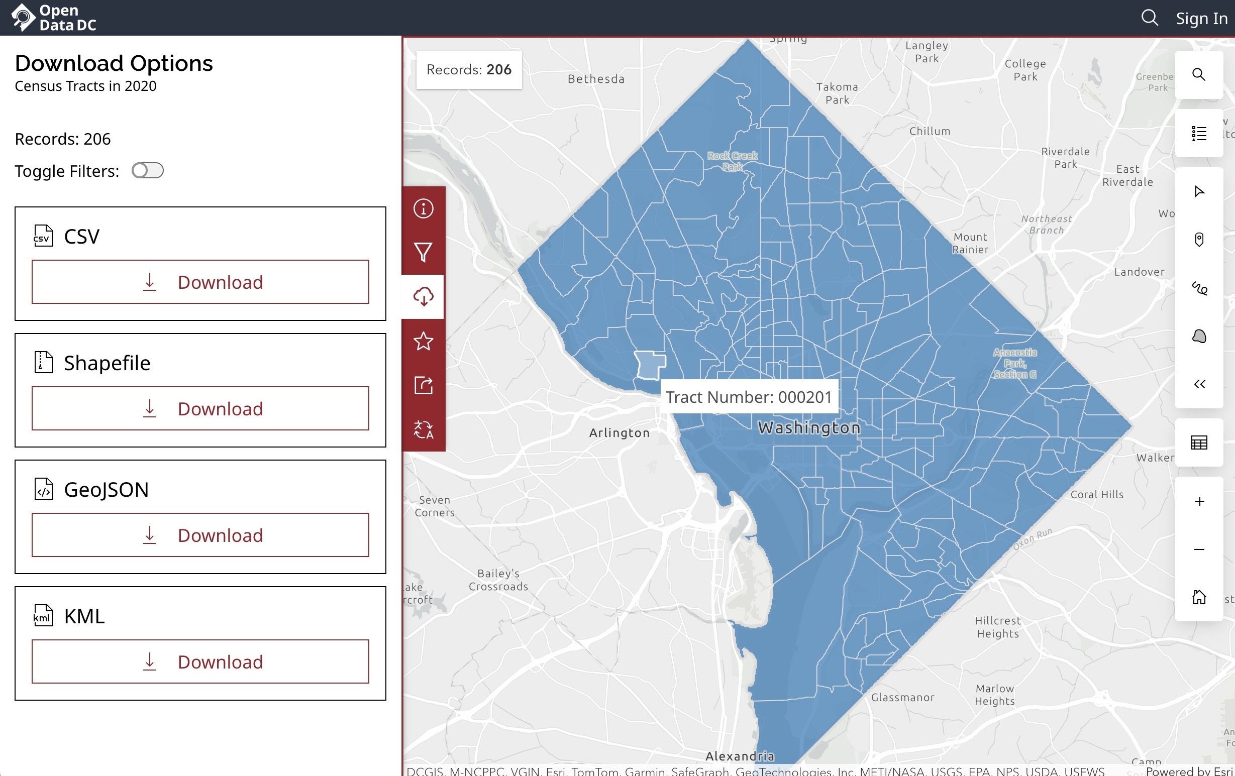
DC Census Tracts (with the Georgetown campus tract highlighted!) from OpenData.DC.gov

Shapefile Anatomy

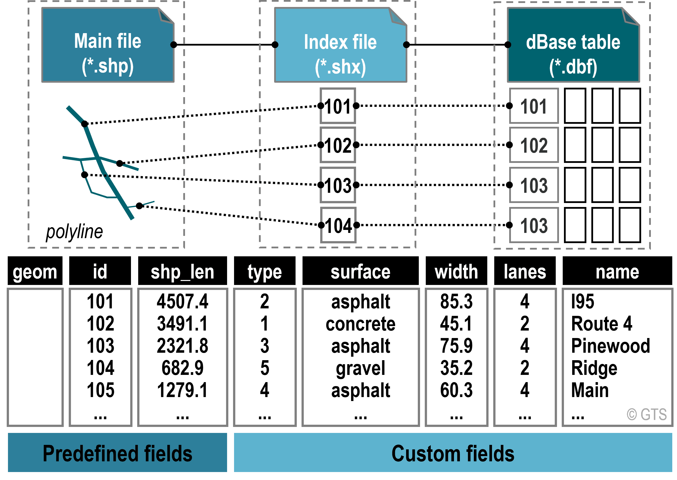
From Rodrigue (2016)

GeoJSON / TopoJSON (.geojson)

• JavaScript Object Notation: General cross-platform format
• Useful when data is too complex for e.g. .csv
• TopoJSON = Memory-efficient GeoJSON
• Bonus: Inline preview on GitHub!

my_data.geojson

{
  "type": "FeatureCollection",
  "features": [
    {
      "type": "Feature",
      "geometry": {
        "type": "Polygon",
        "coordinates": [
          [
            [30, 20], [45, 40],
            [10, 40], [30, 20]
          ]
        ]
      },
      "properties": {
        "color": "green",
        "area": 3565747
      }
    },
    {
      "type": "Feature",
      "geometry": {
        "type": "Polygon",
        "coordinates": [
          [
            [15, 5], [40, 10],
            [10, 20], [5, 10], 
            [15, 5]
          ]
        ]
      },
      "properties": {
        "color": "red",
        "area": 3272386
      }
    }
  ]
}

GeoPackage (.gpkg)

• Open-source (non-proprietary) data format standard

Raster Formats

• GeoTIFF (.tif or .tiff)
  • Based on TIFF format developed at NASA
• NetCDF (.nc4)
  • Used in earth sciences, as format for data sources measured and distributed multiple times per day over large full-country or full-continent areas.

Coordinate Reference Systems (CRS)

• EPSG (European Petroleum Survey Group) Registry: Most common way to specify a CRS

  • For example, 4326 is the EPSG code for the WGS84 coordinate system

• PROJ: Rather than opaque numeric code like EPSG, uses plaintext “proj-strings” containing parameter info: datum, ellipsoid, projection, and units (e.g. meters). Example: PROJ4 code EPSG:4326 is represented as

  +proj=longlat +ellps=WGS84 +datum=WGS84 +no_defs

• WKT: Lengthy but human-readable descriptions

Geospatial Operations 1: Unary Operations

Getting the Geometries

Using rnaturalearth with mapview

set.seed(6805)
library(tidyverse)
library(sf)
library(rnaturalearth)
library(mapview)
source("../dsan-globals/_globals.r")
france_sf <- ne_countries(country = "France", scale = 50)
(france_map <- mapview(france_sf, label = "geounit", legend = FALSE))

Centroid of France

france_cent_sf <- sf::st_centroid(france_sf)
france_map + mapview(france_cent_sf, label = "Centroid", legend = FALSE)

One We Already Saw: Union

Computing the union of all geometries in the sf via sf::st_union()

library(leaflet.extras2)
africa_sf <- ne_countries(continent = "Africa", scale = 50)
africa_union_sf <- sf::st_union(africa_sf)
africa_map <- mapview(africa_sf, label="geounit", legend=FALSE)
africa_union_map <- mapview(africa_union_sf, label="st_union(africa)", legend=FALSE)
africa_map | africa_union_map

Helpful for Rasterizing: BBox

africa_bbox_sf <- sf::st_bbox(africa_sf)
africa_bbox_map <- mapview(africa_bbox_sf, label="st_bbox(africa)", legend=FALSE)
africa_map | africa_bbox_map

Convex Hulls by Country

africa_countries_cvx <- sf::st_convex_hull(africa_sf)
africa_countries_cvx_map <- mapview(africa_countries_cvx, label="geounit", legend=FALSE)
africa_map | africa_countries_cvx_map

Convex Hull of Continent

Use st_union() first:

africa_cvx <- africa_sf |> st_union() |> st_convex_hull()
africa_cvx_map <- mapview(africa_cvx, label="geounit", legend=FALSE)
africa_map | africa_cvx_map

One We Already Saw: Centroids

Computing the centroid of all geometries in the sf via sf::st_centroid()

africa_cents_sf <- sf::st_centroid(africa_sf)
africa_cents_map <- mapview(africa_cents_sf, label="geounit", legend=FALSE)
africa_map | africa_cents_map

Geospatial Operations 2: Binary Operations

Spatial Joins

nc <- system.file("shape/nc.shp", package="sf") |>
  read_sf() |>
  st_transform('EPSG:2264')
gr <- st_sf(
         label = apply(expand.grid(1:10, LETTERS[10:1])[,2:1], 1, paste0, collapse = ""),
         geom = st_make_grid(nc))
gr$col <- sf.colors(10, categorical = TRUE, alpha = .3)
# cut, to verify that NA's work out:
gr <- gr[-(1:30),]
suppressWarnings(nc_j <- st_join(nc, gr, largest = TRUE))
par(mfrow = c(2,1), mar = rep(0,4))
plot(st_geometry(nc_j), border = 'grey')
plot(st_geometry(gr), add = TRUE, col = gr$col)
text(st_coordinates(st_centroid(st_geometry(gr))), labels = gr$label, cex = .85)
# the joined dataset:
plot(st_geometry(nc_j), border = 'grey', col = nc_j$col)
text(st_coordinates(st_centroid(st_geometry(nc_j))), labels = nc_j$label, cex = .7)
plot(st_geometry(gr), border = '#88ff88aa', add = TRUE)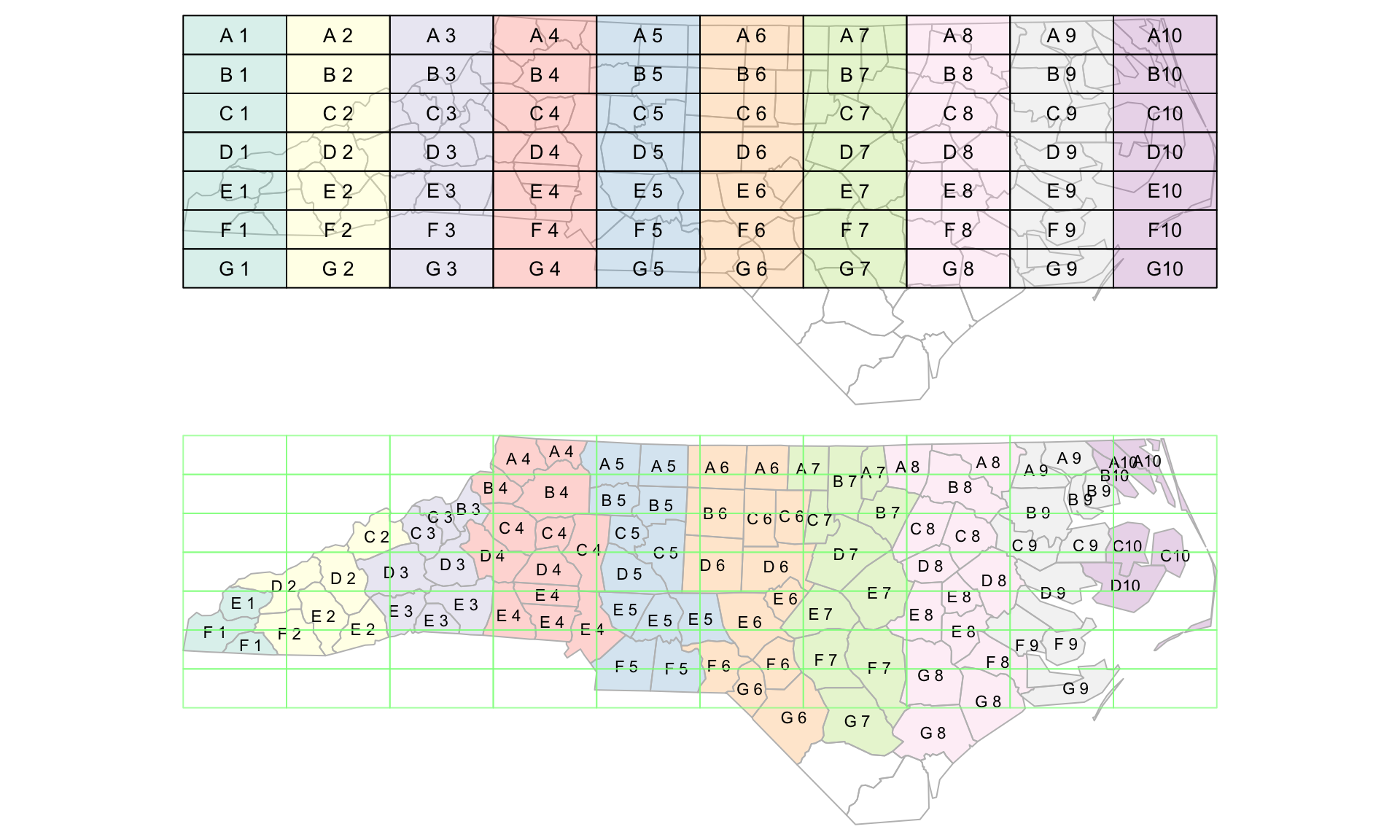

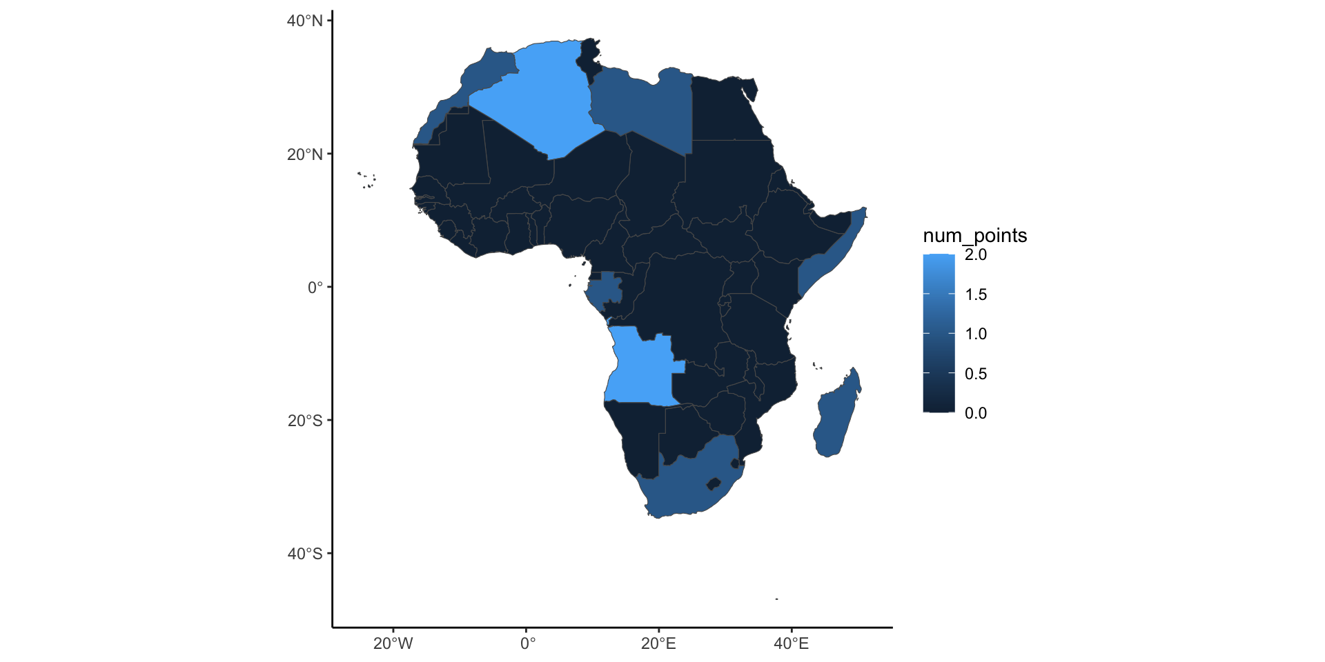
Spatial Sampling

# Sample random points
africa_points_list <- sf::st_sample(africa_union_sf, 10)
africa_points_sf <- sf::st_sf(africa_points_list)
africa_points_map <- mapview(africa_points_sf, label="Random Point", col.regions=cbPalette[1], legend=FALSE)
africa_map + africa_points_map

The “Default” Predicate: st_intersects

countries_w_points <- africa_sf[africa_points_sf,]
mapview(countries_w_points, label="geounit", legend=FALSE) + africa_points_map

Counting with lengths()

country_inter <- sf::st_intersects(africa_sf, africa_points_sf)
# Computes point counts for each polygon
(num_intersections <- lengths(country_inter))

 [1] 0 0 0 0 0 0 0 0 0 1 1 0 0 0 0 0 0 0 0 0 1 0 0 0 0 1 1 0 0 0 0 0 0 0 1 0 0 0
[39] 0 0 0 0 0 0 0 0 0 0 0 0 0 0 2 2

africa_sf <- africa_sf |> mutate(
  num_points = num_intersections
) |> arrange(geounit)
africa_sf |> select(geounit, num_points) |> head()

geounit	num_points	geometry
Algeria	2	MULTIPOLYGON (((8.576563 36…
Angola	2	MULTIPOLYGON (((13.07275 -4…
Benin	0	MULTIPOLYGON (((1.622656 6….
Botswana	0	MULTIPOLYGON (((25.25879 -1…
Burkina Faso	0	MULTIPOLYGON (((0.9004883 1…
Burundi	0	MULTIPOLYGON (((30.55361 -2…

Plotting with mapview

mapview(africa_sf, zcol="num_points")

Plotting with ggplot2

Since we’re starting to get into data attributes rather than geometric features, switching to ggplot2 is recommended!

africa_sf |> ggplot(aes(fill=num_points)) +
  geom_sf() +
  theme_classic()

Getting Fancier…

• To do fancier geospatial operations, we’ll need to start overthinking the different possible relationships between two or more geometries!
• To this end: predicates

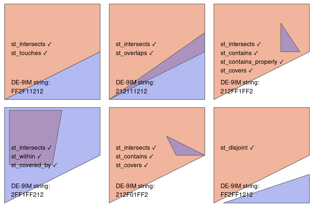
DE-9IM Strings

library(sf)
polygon <- po <- st_polygon(list(rbind(c(0,0), c(1,0), c(1,1), c(0,1), c(0,0))))
p0 <- st_polygon(list(rbind(c(-1,-1), c(2,-1), c(2,2), c(-1,2), c(-1,-1))))
line <- li <- st_linestring(rbind(c(.5, -.5), c(.5, 0.5)))
s <- st_sfc(po, li)

par(mfrow = c(3,3))
par(mar = c(1,1,1,1))

# "1020F1102"
# 1: 1
plot(s, col = c(NA, 'darkgreen'), border = 'blue', main = expression(paste("I(pol)",intersect(),"I(line) = 1")))
lines(rbind(c(.5,0), c(.5,.495)), col = 'red', lwd = 2)
points(0.5, 0.5, pch = 1)

# 2: 0
plot(s, col = c(NA, 'darkgreen'), border = 'blue', main = expression(paste("I(pol)",intersect(),"B(line) = 0")))
points(0.5, 0.5, col = 'red', pch = 16)

# 3: 2
plot(s, col = c(NA, 'darkgreen'), border = 'blue', main = expression(paste("I(pol)",intersect(),"E(line) = 2")))
plot(po, col = '#ff8888', add = TRUE)
plot(s, col = c(NA, 'darkgreen'), border = 'blue', add = TRUE)

# 4: 0
plot(s, col = c(NA, 'darkgreen'), border = 'blue', main = expression(paste("B(pol)",intersect(),"I(line) = 0")))
points(.5, 0, col = 'red', pch = 16)

# 5: F
plot(s, col = c(NA, 'darkgreen'), border = 'blue', main = expression(paste("B(pol)",intersect(),"B(line) = F")))

# 6: 1
plot(s, col = c(NA, 'darkgreen'), border = 'blue', main = expression(paste("B(pol)",intersect(),"E(line) = 1")))
plot(po, border = 'red', col = NA, add = TRUE, lwd = 2)

# 7: 1
plot(s, col = c(NA, 'darkgreen'), border = 'blue', main = expression(paste("E(pol)",intersect(),"I(line) = 1")))
lines(rbind(c(.5, -.5), c(.5, 0)), col = 'red', lwd = 2)

# 8: 0
plot(s, col = c(NA, 'darkgreen'), border = 'blue', main = expression(paste("E(pol)",intersect(),"B(line) = 0")))
points(.5, -.5, col = 'red', pch = 16)

# 9: 2
plot(s, col = c(NA, 'darkgreen'), border = 'blue', main = expression(paste("E(pol)",intersect(),"E(line) = 2")))
plot(p0 / po, col = '#ff8888', add = TRUE)
plot(s, col = c(NA, 'darkgreen'), border = 'blue', add = TRUE)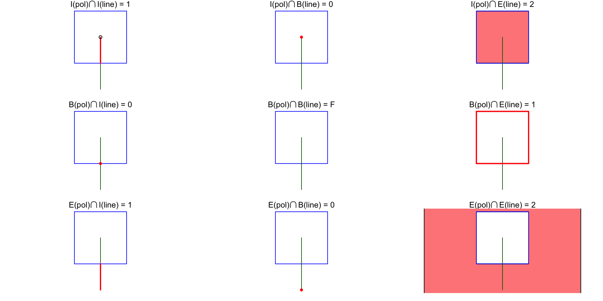

• The predicate equals corresponds to the DE-9IM string "T*F**FFF*". If any two geometries obey this relationship, they are (topologically) equal!

References

Rodrigue, Jean-Paul. 2016. The Geography of Transport Systems. Taylor & Francis.