Week 1: Introduction to GIS

PPOL 6805 / DSAN 6750: GIS for Spatial Data Science
Fall 2025

Jeff Jacobs

jj1088@georgetown.edu

Wednesday, August 26, 2026

Welcome to The Wonderful World of GIS!

Your Final Project

Unit 1: Maps

• Your least favorite part of the course (per survey 😜)
• My favorite part of the course (because I love overthinking things)
• My goal given survey results: Let’s think of this unit like learning languages for expressing spatial information:

Temporal Information	Spatial Information
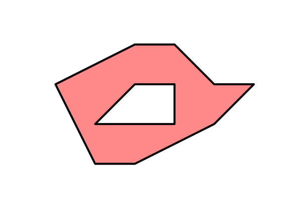
\(\Rightarrow\) 22.5 seconds	\(\Rightarrow\) POLYGON ((2 1, 3 1, 5 2, 6 3, 5 3, 4 4, 3 4, 1 3, 2 1),(2 2, 3 3, 4 3, 4 2, 2 2))

• I think you’ll be surprised at how, complexity of geospatial/spatio-temporal data \(\implies\) need for programming-language-independent representations

Unit 2: Using Code to Make Maps

• (More on this in Prereqs section below!)
• Given representations from Part 1, the task of coding becomes task of finding “best” library for loading/manipulating/plotting them
  • Where “best” = best for you!
• In R: sf and friends (tidyverse)
• In Python: geopandas

Unit 3: Spatial Data Science

• Drawing inferences about spatial phenomena
• The meat of the course
• How can we write code (Unit 2) to analyze a map (Unit 1) so as to…
  • Discover patterns (EDA: Exploratory Data Analysis) or
  • Test hypotheses (CDA: Confirmatory Data Analysis)

Unit 4: Applications / Final Project

• Take everything you’ve learned in Units 1-3 and use them to learn something about the world!
• Public Policy: Which counties are most in need of more transportation infrastructure?
• Urban Planning: Which neighborhoods are most in need of a new bus stop?
• Epidemiology: What properties of a region make it more/less susceptible to infectious diseases? Where should we intervene to “cut the chain” of a disease vector?

Who Am I? Why Am I Teaching You?

• Started out as PhD student in Computer Science
  • UCLA: Algorithmic Game Theory
  • Stanford (MS): Economic Network Analysis
• Ended up with PhD in Political Economy
  • Columbia: “Computational Political Theory”

My GIS Adventures

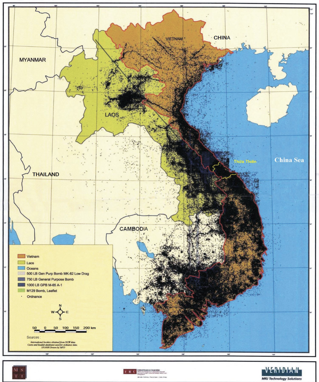
• High school project: mine defusal in Indochina
• As a Telecommunications Engineer for Huawei (HKUST)
• As an Urban Economist at UC Berkeley
  • Used, e.g., Google Maps API to evaluate effects of Suburbanization of Poverty

My GIS 🤯 Moment

• Horrors of “Vietnam War” did not end in 1975…
• Casualties from unexploded ordnance (cluster bombs) continue to devastate the region, over 220,000 victims:
  • >105K in Vietnam
  • >50K in Laos
  • >65K in Cambodia

From Robert (2016)

Huawei: Optimizing Cell Tower Placement

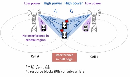
From LTE 4G/5G Self-Organizing Networks  

The Suburbanization of Poverty

• Since 2008, a person living in poverty in the US is more likely to be in a suburb than an “inner city”
• What does this mean for…
  • Access to Food / Public Services?
  • Finding a job \(\leadsto\) Commuting?
• My job: computing “suburban accessibility indices”
• Does commuting = straight line distance?

“Distance” vs. Distance!

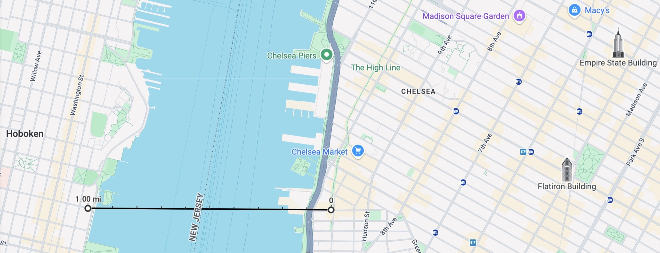
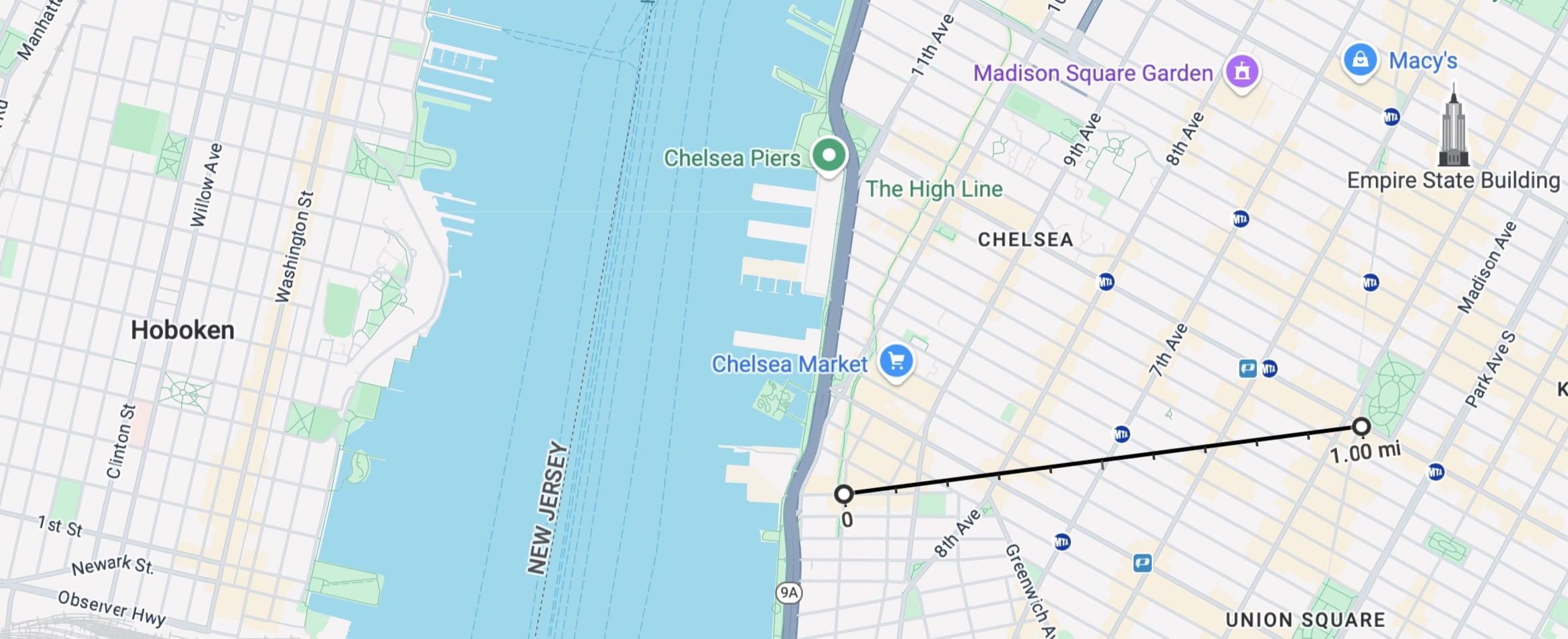
You’ve just been hired as a fine art curator at The Whitney… Congratulations!

Commuting 1 mile to the Whitney
Also commuting 1 mile to the Whitney

Why Should You Care About GIS?

• As a Human
• As a Data Scientist
• As a Public Policy Expert

As Humans

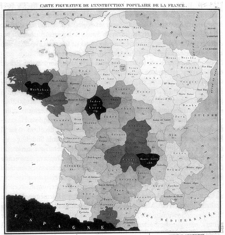
• To understand the world around you!

Charles Dupin, Carte figurative de l’instruction populaire de la France (1826)

• \(\implies\) Crucial landmark in the genesis of social science

As Data Scientists

• All data scientists are expected to know how to analyze “standard” types of data: tabular, numeric data (think spreadsheets)
• However, you can differentiate yourself in the scary scary job market by developing a particular focus on some “non-standard” type:

Hello Mrs. Google Meta OpenAI, yes, indeed, I have a wealth of experience working with [text data / temporal data / signal processing / geospatial data]. This job will be no problem for me.

As Public Policy Experts

• Oftentimes, all it takes is one map to see why a policy has failed 😱

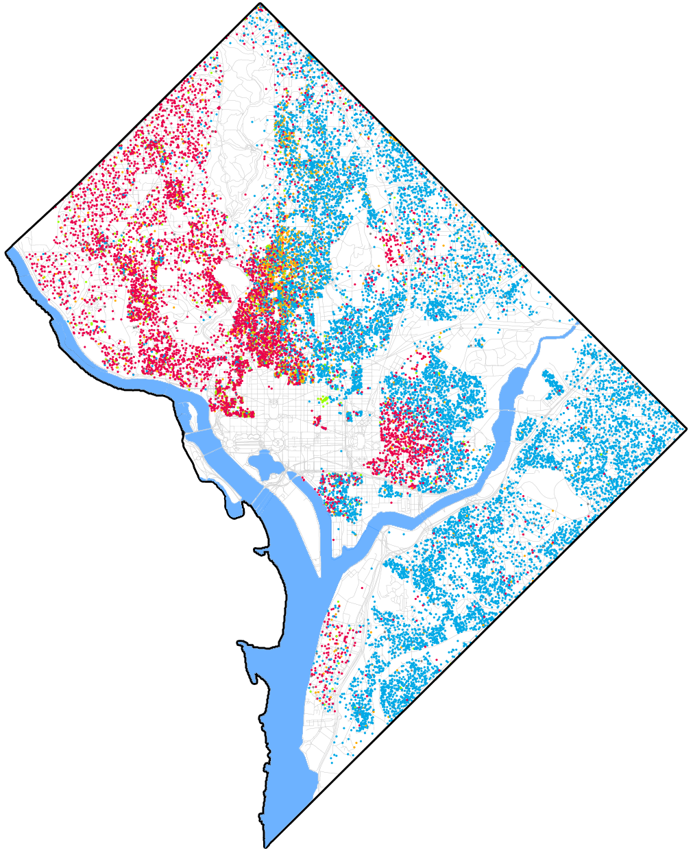
Who can guess what this map represents? (Source)

http://www.radicalcartography.net/index.html?chicagodots, then adapted to DC: “[Eric Fisher] was astounded by Bill Rankin’s map of Chicago’s racial and ethnic divides and wanted to see what other cities looked like mapped the same way. To match his map, Red is White, Blue is Black, Green is Asian, Orange is Hispanic, Gray is Other, and each dot is 25 people. Data from Census 2000. Base map © OpenStreetMap, CC-BY-SA” https://commons.wikimedia.org/wiki/File:Race_and_ethnicity_map_of_Washington,_D.C..png

GIS as an “Umbrella Term”

• Libraries and tools we’ll use: specific systems/methods for geospatial analysis
• GIS is an “umbrella term”, which just vaguely refers to this entire universe of libraries/tools/techniques/approaches

Umbrella Term	Concepts	Specific Skills
Coding	Variables Control Flow Algorithms	Python R JavaScript
GIS	Projections Vector vs. Raster Spatial Data Formats (shapefiles, .geojson)	ArcGIS GeoPandas (Python) sf (R)

ArcGIS…

• For info on Georgetown’s provision of ArcGIS (Online, Pro, and Desktop), see the Library Guide

Ukraine Level-1 Administrative Regions Map (see CDTO talk)

Then… Why Can’t We Just Use ArcGIS?

Analogy from non-geospatial data science:

Text Drawn Map	→	Speadsheet Digital Map	→	Equations Maps w/ArcGIS	→	Code This Class
Start writing info.txt I gave Ana $3, then Ana paid me back $2. [...] Realize there’s regularity/structure 🤔		Start entering info in rows Fr To Amt Bal Me Ana $3 -$3 Ana Me $2 -$1 Realize you’re manually computing things that could be automated 🤔		Start using equations Fr To Amt Bal Me Ana $3 =0-C1 Ana Me $2 =D1-C2 Realize you need fancier equations, and/or need to coordinate with inputs (APIs), outputs (plotting libraries) 🤔		Write code plot_balance.py import pandas as pd df = pd.read_csv(...) calc_weekly_balance() df.plot() Profit 💲💰🤑💰💲

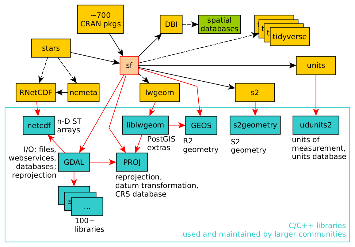
The Spatial Data Science Universe

• We’ll cover key pieces: GDAL (Geospatial Data Abstraction Library), PROJ to convert between projections, GEOS for computational geometry

Course Policy Things

• How To Not Be Scared of Prerequisites
• AI Things
• Learning How To Learn

Pedagogical Principles

• There’s literally no such thing as “intelligence”
• Anyone is capable of learning anything (neural plasticity)
• Growth mindset: “I can’t do this” \(\leadsto\) “I can’t do this yet!”
• The point of a class is learning: understanding something about the world, either (a) For its own sake (end in itself) or (b) Because it’s relevant to something you care about (means to an end)

Our teaching should be governed, not by a desire to make students learn things, but by the endeavor to keep burning within them that light which is called curiosity. (Montessori 1916)

AI and Whatnot

• If you feel like AI things will help you learn something in the course, then use them!
• If you feel like you’re using them as a “crutch”, try to hold yourself accountable for not using it!

Take the time/energy you're using to worry about...	Use it instead to worry about...
AI Policies Collaboration Policies Plagiarism	Learning GIS

On Not Worrying About Prereqs

• I genuinely believe that I can make the course accessible to you, meeting you wherever you’re at, no matter what!
• Everyone learns at their own pace (who says 14 weeks is “correct” amount of time to learn GIS?), and I structure my courses as best as I possibly can to adapt to your pace
• \(\Rightarrow\) Assessments (HW, Midterm) valuable in two ways:
• [Valuable for you] As an accountability mechanism to make sure you’re learn the material (how do we know when we’ve learned something? When we can answer questions about it / use it to accomplish things!)
• [Valuable for me] For assessing and updating pace

R and/or Python and/or JS

• My Geometry vs. Algebra Rant… Euclid’s Elements, Book VI, Proposition 28.
• The problem: Divide a given straight line so that the rectangle contained by its segments may be equal to a given area, not exceeding the square of half the line.

Geometers solved w/geometry (300 BC)…

…Algebraists solved w/algebra (2000 BC)…

\[ \begin{align*} &ax^2 + bx + c = 0 \\ \Rightarrow \; & x_+ = \frac{-b + \sqrt{b^2 - 4ac}}{2a} \end{align*} \]

…From 1637 onwards, whichever is easier! 🤯🤯🤯 (Isomorphism)

Fig 1: Circle with radius 1? Or \((x,y)\) satisfying \(x^2 + y^2 = 1\)?

Learning How To Learn

Fig 2: From The Carter (Documentary)

He’s Literally Extremely Correct!

From Elsevier Osmosis: Spaced Repetition

Let’s Make Some Dang Maps!

Our First Map: Polygons!

library(tidyverse)
library(rmarkdown)
library(sf)
# Load DC tracts data
dc_sf_fpath <- "data/DC_Census_2020/Census_Tracts_in_2020.shp"
dc_sf <- st_read(dc_sf_fpath);

Reading layer `Census_Tracts_in_2020' from data source 
  `/Users/jpj/gtown-local/ppol6805/w01/data/DC_Census_2020/Census_Tracts_in_2020.shp' 
  using driver `ESRI Shapefile'
Simple feature collection with 206 features and 315 fields
Geometry type: POLYGON
Dimension:     XY
Bounding box:  xmin: -8584933 ymin: 4691871 xmax: -8561515 ymax: 4721078
Projected CRS: WGS 84 / Pseudo-Mercator

cols_to_keep <- c(
  "OBJECTID", "TRACT", "GEOID", "ALAND", "AWATER",
  "STUSAB", "SUMLEV", "GEOCODE", "STATE", "NAME",
  "POP100", "HU100", "geometry"
)
dc_sf <- dc_sf |> select(cols_to_keep)

sf Objects

dc_sf is an R object of type sf (short for “simple features”), which extends data.frame by adding a special column named geometry (containing POLYGONs)

class(dc_sf)

[1] "sf"         "data.frame"

dim(dc_sf)

[1] 206  13

rmarkdown::paged_table(dc_sf, options=list(rows.print=6))

What Are These POLYGON Objects?

head(dc_sf)

Simple feature collection with 6 features and 12 fields
Geometry type: POLYGON
Dimension:     XY
Bounding box:  xmin: -8577962 ymin: 4708107 xmax: -8572564 ymax: 4716136
Projected CRS: WGS 84 / Pseudo-Mercator
  OBJECTID  TRACT       GEOID  ALAND AWATER STUSAB SUMLEV     GEOCODE STATE
1        1 002002 11001002002 849376      0     DC    140 11001002002    11
2        2 002101 11001002101 600992      0     DC    140 11001002101    11
3        3 002102 11001002102 725975      0     DC    140 11001002102    11
4        4 002201 11001002201 415173      0     DC    140 11001002201    11
5        5 002202 11001002202 698895    566     DC    140 11001002202    11
6        6 000101 11001000101 199776   5261     DC    140 11001000101    11
                NAME POP100 HU100                       geometry
1 Census Tract 20.02   4072  1532 POLYGON ((-8575655 4714476,...
2 Census Tract 21.01   5687  2335 POLYGON ((-8574745 4715676,...
3 Census Tract 21.02   5099  2221 POLYGON ((-8573824 4715684,...
4 Census Tract 22.01   3485  1229 POLYGON ((-8574654 4714781,...
5 Census Tract 22.02   3339  1454 POLYGON ((-8573792 4714811,...
6  Census Tract 1.01   1406   999 POLYGON ((-8577962 4708867,...

Zoom… Enhance…

Let’s try printing just the first row?

rmarkdown::paged_table(dc_sf[1,])

Printing the special geometry column?

rmarkdown::paged_table(dc_sf[1, "geometry"])

Nope, we’ll have to open the “black box” using the st_coordinates() function from the sf library →

sf::st_coordinates(dc_sf[1,"geometry"])

              X       Y L1 L2
  [1,] -8575655 4714476  1  1
  [2,] -8575655 4714588  1  1
  [3,] -8575655 4714628  1  1
  [4,] -8575655 4714781  1  1
  [5,] -8575655 4714876  1  1
  [6,] -8575636 4714900  1  1
  [7,] -8575622 4714920  1  1
  [8,] -8575613 4714934  1  1
  [9,] -8575595 4714962  1  1
 [10,] -8575564 4715009  1  1
 [11,] -8575519 4715077  1  1
 [12,] -8575502 4715104  1  1
 [13,] -8575452 4715179  1  1
 [14,] -8575408 4715248  1  1
 [15,] -8575362 4715318  1  1
 [16,] -8575359 4715322  1  1
 [17,] -8575320 4715400  1  1
 [18,] -8575294 4715424  1  1
 [19,] -8575272 4715454  1  1
 [20,] -8575268 4715459  1  1
 [21,] -8575242 4715499  1  1
 [22,] -8575237 4715507  1  1
 [23,] -8575226 4715523  1  1
 [24,] -8575221 4715531  1  1
 [25,] -8575205 4715556  1  1
 [26,] -8575198 4715567  1  1
 [27,] -8575190 4715579  1  1
 [28,] -8575167 4715614  1  1
 [29,] -8575142 4715652  1  1
 [30,] -8575132 4715668  1  1
 [31,] -8575116 4715692  1  1
 [32,] -8575105 4715709  1  1
 [33,] -8575094 4715724  1  1
 [34,] -8575069 4715764  1  1
 [35,] -8575031 4715822  1  1
 [36,] -8575021 4715836  1  1
 [37,] -8575008 4715855  1  1
 [38,] -8574983 4715894  1  1
 [39,] -8574959 4715928  1  1
 [40,] -8574954 4715933  1  1
 [41,] -8574952 4715935  1  1
 [42,] -8574943 4715943  1  1
 [43,] -8574939 4715947  1  1
 [44,] -8574907 4715975  1  1
 [45,] -8574904 4715976  1  1
 [46,] -8574901 4715977  1  1
 [47,] -8574898 4715978  1  1
 [48,] -8574893 4715980  1  1
 [49,] -8574889 4715984  1  1
 [50,] -8574886 4715986  1  1
 [51,] -8574883 4715990  1  1
 [52,] -8574857 4716021  1  1
 [53,] -8574802 4716086  1  1
 [54,] -8574783 4716108  1  1
 [55,] -8574779 4716114  1  1
 [56,] -8574778 4716117  1  1
 [57,] -8574775 4716123  1  1
 [58,] -8574774 4716127  1  1
 [59,] -8574775 4716129  1  1
 [60,] -8574776 4716136  1  1
 [61,] -8574735 4716130  1  1
 [62,] -8574724 4716125  1  1
 [63,] -8574719 4716120  1  1
 [64,] -8574720 4716116  1  1
 [65,] -8574721 4716094  1  1
 [66,] -8574721 4716090  1  1
 [67,] -8574724 4716050  1  1
 [68,] -8574730 4715948  1  1
 [69,] -8574736 4715850  1  1
 [70,] -8574742 4715760  1  1
 [71,] -8574743 4715730  1  1
 [72,] -8574744 4715709  1  1
 [73,] -8574744 4715699  1  1
 [74,] -8574745 4715676  1  1
 [75,] -8574745 4715665  1  1
 [76,] -8574744 4715654  1  1
 [77,] -8574744 4715631  1  1
 [78,] -8574742 4715608  1  1
 [79,] -8574742 4715596  1  1
 [80,] -8574741 4715585  1  1
 [81,] -8574737 4715555  1  1
 [82,] -8574736 4715539  1  1
 [83,] -8574733 4715518  1  1
 [84,] -8574731 4715495  1  1
 [85,] -8574726 4715446  1  1
 [86,] -8574721 4715403  1  1
 [87,] -8574720 4715389  1  1
 [88,] -8574718 4715373  1  1
 [89,] -8574713 4715331  1  1
 [90,] -8574706 4715261  1  1
 [91,] -8574705 4715250  1  1
 [92,] -8574703 4715235  1  1
 [93,] -8574699 4715194  1  1
 [94,] -8574695 4715157  1  1
 [95,] -8574688 4715097  1  1
 [96,] -8574687 4715085  1  1
 [97,] -8574670 4714929  1  1
 [98,] -8574669 4714917  1  1
 [99,] -8574669 4714914  1  1
[100,] -8574654 4714781  1  1
[101,] -8574651 4714745  1  1
[102,] -8574638 4714628  1  1
[103,] -8574637 4714615  1  1
[104,] -8574636 4714603  1  1
[105,] -8574634 4714590  1  1
[106,] -8574633 4714578  1  1
[107,] -8574631 4714565  1  1
[108,] -8574630 4714553  1  1
[109,] -8574625 4714503  1  1
[110,] -8574622 4714475  1  1
[111,] -8574616 4714418  1  1
[112,] -8574612 4714382  1  1
[113,] -8574611 4714369  1  1
[114,] -8574608 4714347  1  1
[115,] -8574607 4714336  1  1
[116,] -8574602 4714293  1  1
[117,] -8574601 4714283  1  1
[118,] -8574600 4714275  1  1
[119,] -8574599 4714264  1  1
[120,] -8574586 4714137  1  1
[121,] -8574583 4714111  1  1
[122,] -8574569 4713998  1  1
[123,] -8574562 4713958  1  1
[124,] -8574609 4713959  1  1
[125,] -8574659 4713958  1  1
[126,] -8574695 4713958  1  1
[127,] -8574741 4713958  1  1
[128,] -8574821 4713959  1  1
[129,] -8574901 4713958  1  1
[130,] -8574921 4713996  1  1
[131,] -8574923 4713999  1  1
[132,] -8574946 4714027  1  1
[133,] -8574966 4714053  1  1
[134,] -8574989 4714082  1  1
[135,] -8575017 4714117  1  1
[136,] -8575019 4714120  1  1
[137,] -8575029 4714133  1  1
[138,] -8575049 4714158  1  1
[139,] -8575057 4714171  1  1
[140,] -8575060 4714175  1  1
[141,] -8575062 4714178  1  1
[142,] -8575065 4714181  1  1
[143,] -8575103 4714228  1  1
[144,] -8575122 4714253  1  1
[145,] -8575129 4714261  1  1
[146,] -8575244 4714265  1  1
[147,] -8575259 4714265  1  1
[148,] -8575284 4714264  1  1
[149,] -8575358 4714264  1  1
[150,] -8575432 4714264  1  1
[151,] -8575443 4714264  1  1
[152,] -8575540 4714264  1  1
[153,] -8575639 4714264  1  1
[154,] -8575656 4714264  1  1
[155,] -8575655 4714476  1  1

Working With sf Objects

head(dc_sf$NAME) # Select column by name  

[1] "Census Tract 20.02" "Census Tract 21.01" "Census Tract 21.02"
[4] "Census Tract 22.01" "Census Tract 22.02" "Census Tract 1.01" 

head(dc_sf[,4]) # Select column by number

Simple feature collection with 6 features and 1 field
Geometry type: POLYGON
Dimension:     XY
Bounding box:  xmin: -8577962 ymin: 4708107 xmax: -8572564 ymax: 4716136
Projected CRS: WGS 84 / Pseudo-Mercator
   ALAND                       geometry
1 849376 POLYGON ((-8575655 4714476,...
2 600992 POLYGON ((-8574745 4715676,...
3 725975 POLYGON ((-8573824 4715684,...
4 415173 POLYGON ((-8574654 4714781,...
5 698895 POLYGON ((-8573792 4714811,...
6 199776 POLYGON ((-8577962 4708867,...

And… Actually Displaying the Map!

# We can extract the geometry with the st_geometry function
dc_geo <- st_geometry(dc_sf)

# Plot the geometry with base R's plot() function
plot(dc_geo)

Looking Ahead: Types of Geospatial Data

Key Notation / Definition

• 2-Dimensional “Spatial Process” (Schabenberger and Gotway 2004, 6)

\[ \text{Data} = \left\{Z(\mathbf{s}) \mid \mathbf{s} \in D \subset \mathbb{R}^2\right\} \]

	Geostatistical Data	Lattice/Region Data	Point Pattern
Criteria	Fixed \(D\), Continuous	Fixed \(D\), Discrete	Random subset \(D^* \subseteq D\)
Interest	Infer non-observed parts of \(D\)	Autocorrelation, clustering	Point-generating process
Example	\(N\) trees \(\mathbf{s}_1, \mathbf{s}_2, \ldots, \mathbf{s}_N\), observed within a sample window \(D \subset \mathbb{R}^2\), (\(D\) some finite plot of land) \(Z(\mathbf{s}_i)\): Attribute(s) at site \(\mathbf{s}_i\) Example: Height. \(Z(\mathbf{s}_1) = 500\text{m}\), \(Z(\mathbf{s}_2) = 850\text{m}\), \(\ldots\)	\(Z(\mathbf{s})\) observed over \(N \times N\) grid of plots \(\Rightarrow\) Contiguity, Neighbors (next section of slides!) \(\Rightarrow\) Autocorrelation: Are points around \(\mathbf{s}_i\) likely to have values similar to \(Z(\mathbf{s}_i)\)?	Unknown number of lightning strikes \(\mathbf{s}_1, \mathbf{s}_2, \ldots\) Contrast with geostatistical: all of \(D\) is observed, but what determines the subset \(D^*\) where events occur? “Unmarked”: Just locations “Marked”: Locations+info (e.g., intensity of strike)

Spatial Randomness

Autocorrelation	\(I = -1\)	←	\(I = 0\)	→	\(I = 1\)
Description	Negative Autocorr		No Autocorr		Positive Autocorr
Event at \(\mathbf{s} = (x,y)\) Implies	Less likely to find another point nearby		No information about nearby points		More likely to find another point nearby
Resulting Pattern	Regularity		Reg/Clustered Mix		Clustering
Process(es) Which Could Produce Pattern	1st Order: Random within even-spaced grid 2nd Order: Competition		1st Order: i.i.d. points 2nd Order: i.i.d. distances		1st Order: Tasty food at clust centers 2nd Order: Cooperation
Fixed \(N\)	60		60		60

Complete Spatial Randomness (CSR)

Autocorrelation	\(I = -1\)	←	\(I = 0\)	→	\(I = 1\)
Description	Negative Autocorr		No Autocorr		Positive Autocorr
Event at \(\mathbf{s} = (x,y)\) Implies	Less likely to find another point nearby		No information about nearby points		More likely to find another point nearby
Resulting Pattern	Regularity		Reg/Clustered Mix		Clustering
Process(es) Which Could Produce Pattern	1st Order: Random within even-spaced grid 2nd Order: Competition		1st Order: i.i.d. points 2nd Order: i.i.d. distances		1st Order: Tasty food at clust centers 2nd Order: Cooperation
Fixed Intensity \(\lambda\)	60		60		60
Random \(N\)

References

Montessori, Maria. 1916. Spontaneous Activity in Education: A Basic Guide to the Montessori Methods of Learning in the Classroom. Lulu Press.

Robert, Amélie. 2016. “At the Heart of the Vietnam War: Herbicides, Napalm and Bulldozers Against the A Lưới Mountains.” Journal of Alpine Research | Revue de Géographie Alpine, no. 104–1, 104–1 (April).

Schabenberger, Oliver, and Carol A. Gotway. 2004. Statistical Methods for Spatial Data Analysis. CRC Press.