Week 11: Classification, Final Review
DSUA111: Data Science for Everyone, NYU, Fall 2020
TA Jeff, jpj251@nyu.edu
- This slideshow: https://jjacobs.me/dsua111-sections/week-11
- All materials: https://github.com/jpowerj/dsua111-sections
Outline
I. Classification
- The K-Nearest Neighbors Algorithm
- Evaluating KNN
II. Final Review
- Big Picture Ideas
- Math/Programming Details
Part I: Classification
The K-Nearest Neighbors Algorithm
- Recall from last time:
- Statistics is generally about explanation
- Machine Learning is generally about prediction
- Binary Classification: Given a set of information ("features") about an observation ($X$), predict a yes/no outcome ($y \in \{0,1\}$) for this observation
- Example: Given a count of words in an email, classify it as spam ($y = 1$) or not spam ($y = 0$)
- Multiclass classification: Classify the observation into one of $N$ categories ($y \in \{0, 1, \ldots, N\}$)
- Example: Given a handwritten symbol, classify it as a digit ($y = \{0, 1, \ldots, 9\}$)
- K-Nearest Neighbors Intuition: Find the $K$ most similar observations that we've seen before, and have them "majority vote" on the outcome.
K-Nearest Neighbors Example
- The problem: Given a student's GPA, predict whether or not they will graduate
- Many different potential approaches!
- K-Nearest Neighbor Approach:
- Get a dataset of previous years, students' GPAs and whether or not they graduated
- Find the $K=5$ students with GPA closest to the student of interest
- If a majority of them graduated, predict that the student will graduate. Otherwise, predict that they will not.
Binary Classification with 2 Features
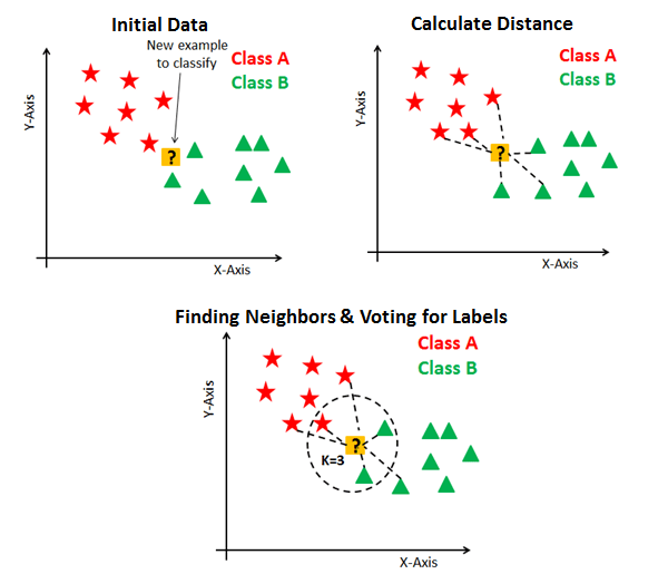
(from https://www.datacamp.com/community/tutorials/k-nearest-neighbor-classification-scikit-learn)
Evaluating KNN
- For binary classification: Seemingly easy, could just compute # correct, # incorrect
- We generally DON'T WANT TO DO THIS (why?)
- Instead, in actual machine learning projects, we use $F$-score:
- Don't worry about the details, the point is that what we really want to do is maximize accuracy ($tp$) subject to a penalty for false positives/negatives.
- This generalizes to multiclass classification: each category has its own $F$-score
Part II: Final Review
Common Misperceptions
0. True or False: The p-value is the probability that the null hypothesis is true.
False. It's the probability that we would obtain a test statistic value this "extreme" if the null hypothesis was true.
1. True or False: A 95% confidence interval means we're 95% confident that the true value of the parameter is between these two values.
False. It's just an interval computed in such a way that if we re-performed the experiment many many times, on average we'd expect the computed interval to contain the true value of the parameter about 95% of the time.
2. True or False: If our p-value is not low enough to meet our significance threshold (say, it's not below 0.05), then we reject the alternative hypothesis and accept the null hypothesis.
False. We never "accept" any hypotheses.
3. True or False: For pd.read_csv("dataset.csv") to work correctly, the dataset.csv file must be in the same folder as our notebook.
True. Otherwise, we have to specify how to "get to" the .csv file from the notebook's folder
4. What about pd.read_csv("../dataset.csv")?
This tells Pandas to look one level above the folder containing the notebook, in the computer's directory tree. (So, if the notebook was located at /home/data_science_projects/my_notebook.ipynb, the above code would look for dataset.csv within the /home folder.
Regression Questions
We're going to load a dataset with GDP per capita (in USD) and level of inequality (as measured by Gini coefficient -- higher values = more unequal) for each country in the world. Then we'll perform a regression with GDP per capita as our independent variable and level of inequality as our dependent variable.
5. Write the equation for our unfitted model in this case
6. What is the null hypothesis that this regression is testing, in terms of this equation?
7. What is the null hypothesis that this regression is testing, in words?
An increase of $1 in GDP per capita is not associated with any change in inequality
8. What is the alternative hypothesis that this regression is testing, in terms of our equation?
9. What is the alternative hypothesis that this regression is testing, in words?
An increase of $1 in GDP per capita is associated with a change in inequality
import pandas as pd
ineq_df = pd.read_csv("gdp_inequality.csv")
ineq_df.rename(columns={'Gini coefficient (World Bank (2016))':'gini',
                        'Output-side real GDP per capita (gdppc_o) (PWT 9.1 (2019))':'gdp'},
               inplace=True)
ineq_df = ineq_df[~pd.isna(ineq_df["gini"])].copy()
ineq_df = ineq_df[~pd.isna(ineq_df["gdp"])].copy()
final_df = ineq_df.groupby("Code").last()
import statsmodels.formula.api as smf
result = smf.ols('gini ~ gdp', data=final_df).fit()
summ = result.summary(); summ.extra_txt = None
summ
10. What does the -0.0002 in the "coef" column of the "gdp" row mean?
An increase of $1 in GDP per capita is associated with a decrease of 0.0002 in Gini coefficient (inequality)
11. Which column do we look at to obtain our p-value?
The column with header P>|t|.
12. True or False: Since the p-value is so low, we can conclude that increases in GDP cause decreases in inequality
False. We should never draw causal conclusions from the results of an OLS regression.
13. Where do we look to obtain the F-statistic for our model?
Towards the top -- the third row, right-hand column, lists the F-statistic (in this case, 24.73)
14. What does this value mean?
This is the test statistic for the hypothesis that all of the coefficients in our model are 0. With reference to our equation above, the null hypothesis for the F-statistic would be
$$H_0: \beta_0 = 0 \text{ and }\beta_1 = 0$$and the alternative hypothesis
$$H_A: \beta_0 \neq 0 \text{ or }\beta_1 \neq 0$$The value 24.73 is high enough that the probability of obtaining an F-statistic as extreme as or more extreme than that is (listed directly underneath the F-statistic in the table) approximately 0. Thus we reject the null hypothesis that all coefficients are zero.
15. True or False: The adjusted $R^2$ value is lower than the $R^2$ value because GDP does not explain much of the variance in Gini coefficient
False. Adjusted $R^2$ is only lower than $R^2$ because it penalizes you for each new independent variable you introduce into the model.
16. How would the interpretation of our coefficient on GDP change if we added another independent variable?
Whereas in the single-variable case we interpret the coefficient as just the effect of GDP on inequality, if we introduced a new independent variable $X_2$ we would have to re-interpret our coefficient on GDP as the effect of GDP on inequality holding $X_2$ constant (or, if we center our variables, like we really should: the effect of GDP on inequality at the average $X_2$ value)
Some Stats
17. If we have an observation $x_5 = 123.45$ in a dataset, and find that the z-score for this value is $z_5 = 2.00$, what does this tell us about the original observation?
It tells us that 123.45 is almost exactly 2 standard deviations above the mean $x$ value.
18. True or False: If the mean of a variable $x$ in our dataset is 50.0 and the standard deviation is 5.0, we know that approximately 68% of the values of $x$ lie within one standard deviation of this mean, i.e., between 45.0 and 55.0.
False. This is important. Because the "68% of the data lie within one standard deviation of the mean" property only holds for normally-distributed observations. The question never stated that the data was normally distributed, thus we can't assume the "68% rule" here.
Some Coding
19. What will the following code output?
for i in range(100):
    if i % 7 == 0:
        print(i)
for i in range(100):
    if i % 7 == 0:
        print(i)
20. What will this code output?
for i in range(100):
    if i / 7 == 0:
        print(i)
for i in range(100):
    if i / 7 == 0:
        print(i)
21. How many times will the following code print `"hello!"?
i = 0
while i < 4:
    for j in range(2):
        print("hello!")
    i = i + 1
i = 0
while i < 4:
    for j in range(2):
        print("hello!")
    i = i + 1
22. How many times will the following code print "hello!"?
i = 0
while i < 4:
    for j in range(i):
        print("hello!")
    i = i + 1
i = 0
while i < 4:
    for j in range(i):
        print("hello!")
    i = i + 1
Returning to our DataFrame...
final_df.head()
23. True or False: The following code permanently renames the "Total population" column so it is henceforth named "pop"
final_df.rename(columns={'Total population (Gapminder, HYDE & UN)':'pop'})
final_df.head()
final_df.rename(columns={'Total population (Gapminder, HYDE & UN)':'pop'}, inplace=True)
final_df.head()
24. Say we make a new variable high_gdp which is 1 if GDP is greater than $10000 and 0 otherwise. What type of variable (not data type) is high_gdp?
It is a [binary] ordinal variable, since there is a natural ordering (since we know countries with high_gdp = 0 have lower GDPs than countries with high_gdp = 1).
final_df['high_gdp'] = final_df['gdp'].apply(lambda x: 1 if x > 10000 else 0)
final_df.head()
25. Say we filled in the Continent column, so that e.g. Africa = 0, Asia = 1, South America = 2, North America = 3, Europe = 4, Oceania = 5. What type of variable (not data type) would Continent be in this case?
In this case Continent would be a categorical variable, not an ordinal variable, since there is no natural ordering of the values. We could just as easily have labeled the continents so that Europe = 0, Oceania = 1, Asia = 2, Africa = 3, North America = 4, South America = 5, without losing any information that this variable is supposed to hold.
sorted_df = final_df.sort_values(by="gini").copy()
us_gini = sorted_df.loc["USA"]["gini"]
us_gini
import numpy as np
sorted_df['gini_vs_us'] = sorted_df['gini'] - us_gini
sorted_df.iloc[83:95]
25. If we only knew the US's gini coefficient (and not its GDP), and we used the K-Nearest Neighbors algorithm with $K = 5$ to try and predict whether it was low or high GDP, which would we predict?
- 1st closest neighbor: Turkmenistan (low GDP)
- 2nd closest neighbor: Morocco (low GDP)
- 3rd closest neighbor: Madagascar (low GDP)
- 4th closest neighbor: Russia (high GDP)
- 5th closest neighbor: Senegal (low GDP)
4 out of 5 are low GDP $\implies$ we predict low GDP for US
26. What about with $K = 7$?
(The above 5 closest neighbors, plus:)
- 6th closest neighbor: Trinidad and Tobago (low GDP)
- 7th closest neighbor: Uruguay (high GDP)
5 out of 7 are low GDP $\implies$ we predict low GDP for US again
27. Why do we always pick odd numbers as values for $K$?
Because we need to take a majority vote of the $K$ neighbors, so odd numbers ensure that we won't encounter any ties.