Week 9: Linear Regression!
DSUA111: Data Science for Everyone, NYU, Fall 2020
TA Jeff, jpj251@nyu.edu
- This slideshow: https://jjacobs.me/dsua111-sections/week-09
- All materials: https://github.com/jpowerj/dsua111-sections
Overview
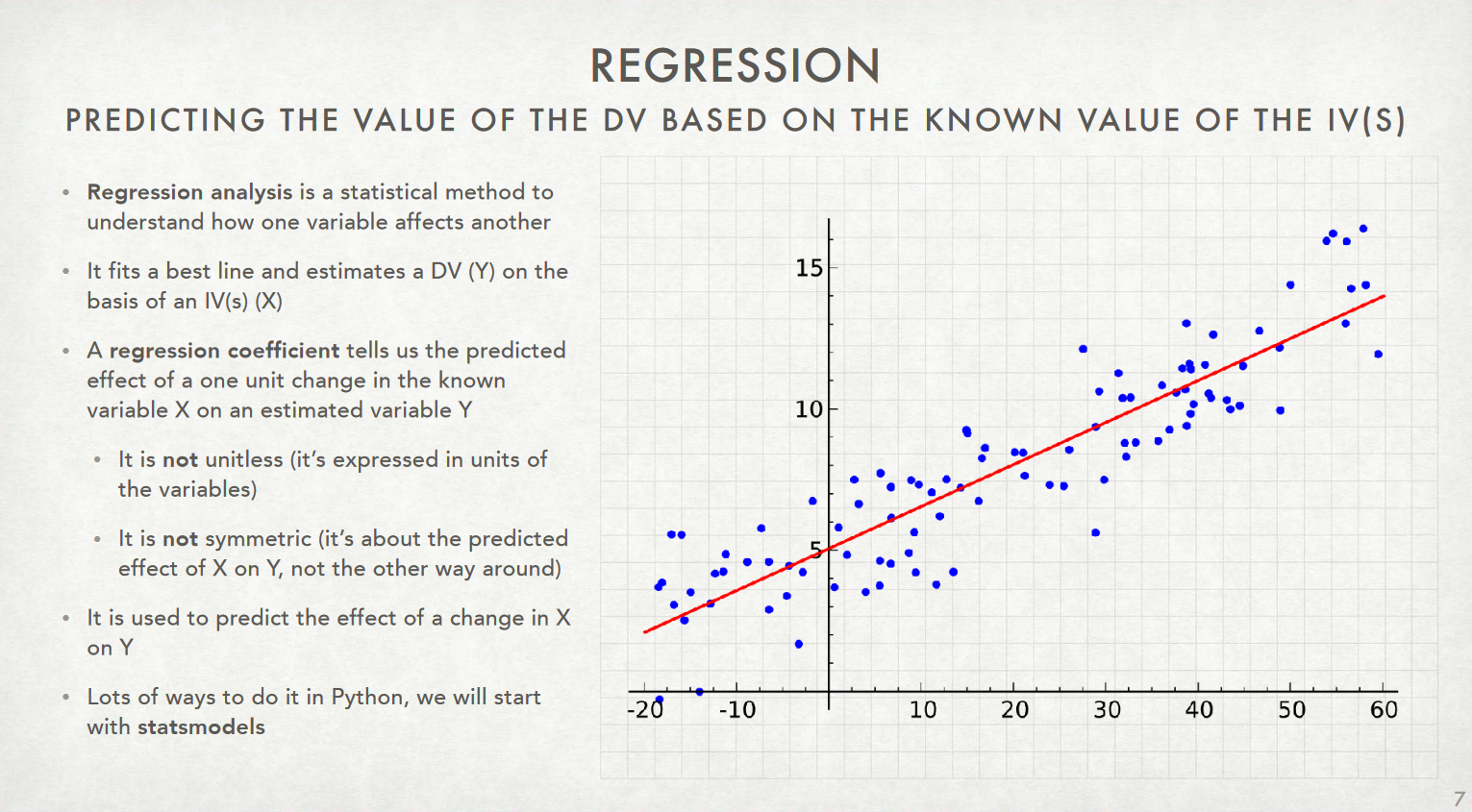
- Regression in General: What it is and what it isn't
- Ordinary Least Squares (OLS) Regression
This is the most important topic in the course, practically speaking
- All the fancy machine learning / AI / neural net methods, they are all glorified regressions
The "best fit" line: make sure you check your intuition!

When given this sort of scatterplot (without any lines superimposed) and asked to draw the regression line of $y$ on $x$, students tend to draw the principal component line shown in Figure 4.2a. However, for the goal of predicting $y$ from $x$, or for estimating the average of $y$ for any given value of $x$, the regression line is in fact better--even if it does not appear so at first.
The superiority of the regression line for estimating the average of $y$ given $x$ can be seen from a careful study of Figure 4.2.
The "best fit" line: make sure you check your intuition!
For example, consider the points at the extreme left of either graph. They all lie above the principal components line but are roughly half below and half above the regression line. Thus, the principal component line underpredicts $y$ for low values of $x$.
Similarly, a careful study of the right side of each graph shows that the principal component line overpredicts $y$ for high values of $x$.
In contrast, the regression line again gives unbiased predictions, in the sense of going through the average value of $y$ given $x$.
(Gelman and Hill, "Data Analysis Using Regression and Multilevel/Hierarchical Models", 58)
Ordinary Least Squares (OLS) Regression: The Model
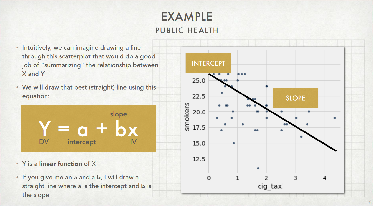
This is the non-"fitted" model, since we don't yet know the precise values of $a$ or $b$
Ordinary Least Squares (OLS) Regression: The Fitted Model
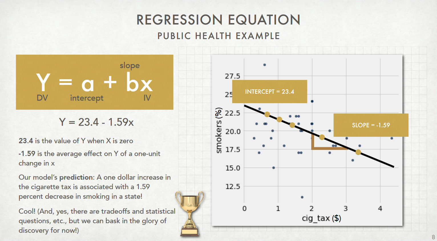
By estimating the parameters of our model using the data in the dataset, we obtain $a = 23.4$ and $b = -1.59$

Regression in Python
import statsmodels.formula.api as smf
The Dataset: Colonial History and Life Expectancy
import pandas as pd
import numpy as np
colonial_df = pd.read_csv("colonial_life_expectancy.csv")
colonial_df
Exploratory Data Analysis
- NOTE: YOU ACTUALLY DO NEED TO DO THIS IRL...
import matplotlib.pyplot as plt
plt.boxplot(colonial_df['life_exp'], vert=False)
plt.xlabel("Life Expectancy (Years)")
# https://matplotlib.org/3.1.1/api/_as_gen/matplotlib.pyplot.tick_params.html
plt.tick_params(axis='y', which='both', left=False, labelleft=False)
plt.show()

Outliers?
colonial_df.sort_values(by='life_exp')
(btw, "Lesotho" is pronounced "Leh-Soo-Too"... fun fact)
Scatterplottin
plt.scatter(colonial_df['yrs_since_ind'], colonial_df['life_exp'])
plt.xlabel("Year Since Independence")
plt.ylabel("Life Expectancy (Years)")
plt.show()

(sidebar: for variables with skewed distributions like years since independence, you really should take the log to "de-skew" them)
plt.scatter(np.log(colonial_df['yrs_since_ind']), colonial_df['life_exp'])
plt.xlabel("Log(Year Since Independence)")
plt.ylabel("Life Expectancy (Years)")
plt.show()

Before we estimate the model, remember what our hypotheses are!
- $H_0$: Changes in the independent variable have no effect on the dependent variable
- i.e., $\beta_1 = 0$
- So, in our case: number of years since independence has no effect on life expectancy
- $H_A$: Changes in the independent variable have some (nonzero) effect on the dependent variable
- i.e., $\beta_1 \neq 0$
- In our case: number of years since independence has an effect on life expectancy
- (Remember our model: $Y_i = \beta_0 + \beta_1X_i + \varepsilon_i$)
- $\textsf{LifeExpectancy}_i = \beta_0 + \beta_1\textsf{YrsSinceIndependence}_i + \varepsilon_i$
results = smf.ols('life_exp ~ yrs_since_ind', data=colonial_df).fit()
(Why do we have to add .fit()?)
summary = results.summary()
summary.extra_txt = None; summary
import seaborn as sns
sns.regplot(x='yrs_since_ind', y='life_exp', data=colonial_df)
plt.title("All Countries")
plt.xlabel("Years Since Independence")
plt.ylabel("Life Expectancy (Years)")
plt.show()

Appendix I: Removing Outliers
- Sketchy, but in this case we have a historical reason for removing outliers: we can revise our population of interest to be countries that achieved independence since the 1648 Treaty of Westphalia, which (long story short) inaugurated the era of the sovereign nation-state
tw_df = colonial_df[colonial_df['yrs_since_ind'] < 368].copy()
print("Number of countries before dropping outliers: " + str(len(colonial_df)))
print("Number of countries after dropping outliers: " + str(len(tw_df)))
plt.scatter(tw_df['yrs_since_ind'], tw_df['life_exp'])
plt.show()

results_tw = smf.ols('life_exp ~ yrs_since_ind', data=tw_df).fit()
tw_summary = results_tw.summary()
tw_summary.extra_txt = None; tw_summary
import seaborn as sns
sns.regplot(x='yrs_since_ind', y='life_exp', data=tw_df)
plt.title("Post-Westphalia Countries")
plt.xlabel("Years Since Independence")
plt.ylabel("Life Expectancy (Years)")
plt.show()

Appendix II: ...You really should log the skewed variables
colonial_df['log_yrs_since_ind'] = colonial_df['yrs_since_ind'].apply(np.log)
results_log = smf.ols('life_exp ~ log_yrs_since_ind', data=colonial_df).fit()
summary_log = results_log.summary()
summary_log.extra_txt = None; summary_log
import seaborn as sns
sns.regplot(x='log_yrs_since_ind', y='life_exp', data=colonial_df)
plt.title("All Countries")
plt.xlabel("Log(Years Since Independence)")
plt.ylabel("Life Expectancy (Years)")
plt.show()

(and now with just the post-Westphalia countries)
tw_df['log_yrs_since_ind'] = tw_df['yrs_since_ind'].apply(np.log)
results_tw_log = smf.ols('life_exp ~ log_yrs_since_ind', data=tw_df).fit()
results_summary = results_tw_log.summary()
results_summary.extra_txt = None; results_summary
import seaborn as sns
sns.regplot(x='log_yrs_since_ind', y='life_exp', data=tw_df)
plt.title("Post-Westphalia Countries")
plt.xlabel("Log(Years Since Independence)")
plt.ylabel("Life Expectancy (Years)")
plt.show()
