Week 8: Hypothesis Testing, Correlation vs. Causation
DSUA111: Data Science for Everyone, NYU, Fall 2020
TA Jeff, jpj251@nyu.edu
- This slideshow: https://jjacobs.me/dsua111-sections/week-08
- All materials: https://github.com/jpowerj/dsua111-sections
Outline
- Hypothesis Testing Overview
- Testing Coins
- Null vs. Alternative Hypotheses
- Test Statistics
- The Normal Distribution
- Correlation vs. Causation
Hypothesis Testing Overview
tl;dr
- If your theory was true, what would the data look like?
- Now compare that to the actual, observed data
Testing Coins
Example: I walk up to you and say "Hey, wanna gamble? We'll each put in a dollar, then I'll flip this coin. Heads I get the \$2, tails you get the \\$2"
- Xavier's Theory: I think the coin is fair. Heads and tails will come up about the same number of times
- Yasmin's Theory: I don't trust this guy, I think heads will come up more often than tails
"Suit yourself -- here, I'll let you flip it 100 times and then draw your own conclusions about whether it's fair or not!"
What do the two theories predict in terms of the outcome of a series of coin flips?
x_predictions = [0.5, 0.5]
y_predictions = [0.25, 0.75]

import matplotlib.pyplot as plt
def plot_prediction(prediction, who):
    plt.bar([0,1], prediction)
    plt.ylim([0,1])
    plt.title(f"{who}'s coin flip prediction")
    plt.show()
plot_prediction(x_predictions, "Xavier")

plot_prediction(y_predictions, "Yasmin")

- Data:
from collections import Counter
import pandas as pd
import numpy as np
import secret_coin
np.random.seed(123)

def do_coin_flips(N):
    coin_flips = np.array([secret_coin.flip() for i in range(N)])
    return coin_flips

def get_flip_distributions(x_predictions, y_predictions, results):
    flip_counter = Counter(results)
    flip_counts = np.array([flip_counter[0], flip_counter[1]]) / len(results)
    flip_df = pd.DataFrame({'outcome':["Tails","Heads"],'p':flip_counts,'which':['Actual outcome','Actual outcome']})
    x_pred_df = pd.DataFrame({'outcome':["Tails","Heads"],'p':x_predictions,'which':["Xavier's prediction","Xavier's prediction"]})
    y_pred_df = pd.DataFrame({'outcome':["Tails","Heads"],'p':y_predictions,'which':["Yasmin's prediction","Yasmin's prediction"]})
    full_df = pd.concat([flip_df, x_pred_df, y_pred_df]).reset_index()
    return full_df
flips_100 = do_coin_flips(100)
flips_100
dist_df = get_flip_distributions(x_predictions, y_predictions, flips_100)
dist_df
plt.bar([0,1], [dist_df.iloc[0]['p'],dist_df.iloc[1]['p']])
plt.title("Actual observed flips (N=100)")
plt.ylim([0,1])
plt.show()

But... how wrong is our prediction?
import seaborn as sns; sns.set_style("whitegrid")
def plot_distributions_a(dist_df):
    g = sns.catplot(data=dist_df, kind="bar",x="outcome", y="p", hue="which")
    g.despine(left=True)
    g.set_axis_labels("Outcome", "P(outcome)")
    g.legend.set_title("")
    g.set(ylim=(0,1))
plot_distributions_a(dist_df)

def plot_distributions_b(dist_df):
    g = sns.catplot(
        data=dist_df, kind="bar",
        x="which", y="p", hue="outcome"
    )
    g.despine(left=True)
    g.set_axis_labels("Which Distribution?", "P(outcome)")
    g.legend.set_title("Outcome")
    g.set(ylim=(0,1))
plot_distributions_b(dist_df)

Hmm... that actual outcome still looks kinda sketchy. Let's try one more time
flips_100_2 = do_coin_flips(100)
flips_100_2
dist_df2 = get_flip_distributions(x_predictions, y_predictions, flips_100_2)
dist_df2
plot_distributions_a(dist_df2)

plot_distributions_b(dist_df2)

So, we need to formalize how to measure how good or bad a prediction is.
Enter... statistics!
Null vs. Alternative Hypotheses
- Null Hypothesis ($H_0$): The skeptical hypothesis... "Nothing interesting is going on here, any patterns were simply due to chance"
- The coin is not weird. $P(\text{heads}) = 0.5$
- Alternative Hypothesis ($H_A$): Something other than chance is generating the pattern we observe
- The coin is loaded! $P(\text{heads}) \neq 0.5$
ONLY TWO POSSIBLE CONCLUSIONS FROM YOUR HYPOTHESIS TEST
- "We reject the null hypothesis"
- if it seems sufficiently unlikely that the patterns in the data were produced simply due to chance
- "We fail to reject the null hypothesis"
- otherwise
Test Statistic
- Computed from the observed data
- A measure of how reasonable our alternative hypothesis is for explaining this data
- I think of it like: a measure of "weirdness" -- should get larger the more "suspicious" the data is
- e.g., for a sequence of dice rolls, should be small if most sides come up ~1/6th of the time, but very high if only 6 ever comes up
Unfair Coin Detection Statistic
- Idea: (number of heads) - (number of tails)
This is the number we were looking for before! It allows us to measure "unfairness" of the coin:
- Fair coins should produce test statistics close to 0 on average, while
- Coins biased towards heads will produce test statistics larger than 0 on average
So, how bad were our coin flip predictions?
def test_stat_a(coin_flips):
    # Num heads - num tails
    num_heads = len([f for f in coin_flips if f == 1])
    num_tails = len([f for f in coin_flips if f == 0])
    return num_heads - num_tails
print(test_stat_a(do_coin_flips(100)))
print(test_stat_a(do_coin_flips(100)))
What would this test statistic look like if the coin was actually fair?
def fair_coin_flips(N):
    return np.array([np.random.binomial(1, 0.5) for i in range(N)])
print(test_stat_a(fair_coin_flips(100)))
print(test_stat_a(fair_coin_flips(100)))
Testing Procedure
- We'll consider a trial to be a sequence of $N=100$ coin flips.
- We'll perform 1000 trials with a fair coin, and for each trial we'll record what the test statistic is
- Once we finish, we'll look at the distribution of test statistics that were generated from flips of the fair coin
test_stats = []
for trial_num in range(1000):
    test_stats.append(test_stat_a(fair_coin_flips(100)))
# Turn it into a NumPy array so we can do fancy math stuff with it
test_stats = np.array(test_stats)
plt.hist(test_stats)
plt.show()

So... now we do 100 flips of our secret coin and see where it falls on this distribution!
secret_coin_results = do_coin_flips(100)
sc_stat = test_stat_a(secret_coin_results)
sc_stat
plt.hist(test_stats)
plt.vlines(sc_stat, 0, 250, color='red')
plt.show()

p-values
- You should always have this plot in your head when thinking about p-values.
- The p-value is just the proportion of test statistics generated from a true null hypothesis (in this case, with a fair coin) that are as extreme or more extreme than the test statistic generated from the observed data
- In this case,
sum(test_stats >= sc_stat) / len(test_stats)
246 out of the 1000 trials of 100 fair coin flips, 24.6%, produced test statistics as extreme or more extreme than 8, so our p-value is 0.246
Increasing the Sample Size
- As of now, the test statistic for our observed sequence of secret-coin flips seems like it could easily be generated by chance.
- If we want to be more confident, we'll need to increase the sample size. This time, let's consider a trial to be 500 coin flips, and re-do our testing procedure
test_stats_500 = []
for i in range(1000):
    coin_flips = fair_coin_flips(500)
    test_stat = test_stat_a(coin_flips)
    test_stats_500.append(test_stat)
test_stats_500 = np.array(test_stats_500)
plt.hist(test_stats_500)
plt.show()

And now we do 500 flips of the secret coin, compute the test statistic for this sequence, and see where it lies on that histogram
secret_coin_results_500 = do_coin_flips(500)
sc_stat_500 = test_stat_a(secret_coin_results_500)
sc_stat_500
plt.hist(test_stats_500)
plt.vlines(sc_stat_500, 0, 200, color='red')
plt.show()

sum(test_stats_500 >= sc_stat_500) / len(test_stats_500)
Ok, now it looks suspicious -- the test statistic for the 500 secret coin flips is way higher than any test statistic produced by 500 flips of a known-fair coin
🤔🤔🤔
So our p-value here would be 0: 0 out of the 1000 fair-coin trials produced test statistics this high or higher!
Alternative Test Statistics
- Remember: the statistic we used is not the only possible test statistic!
- We make up/choose the test statistic that can best help us "detect" not-by-chance data
def test_stat_b(coin_flips):
    # The squared difference in predicted probabilities
    num_heads = len([f for f in coin_flips if f == 1])
    num_tails = len([f for f in coin_flips if f == 0])
    return (num_heads - num_tails) ** 2
test_stats_b = []
for trial_num in range(1000):
    test_stats_b.append(test_stat_b(fair_coin_flips(100)))
test_stats_b = np.array(test_stats_b)
plt.hist(test_stats_b)
plt.show()

Now let's place our observed data on this plot
sc_stat_b = test_stat_b(secret_coin_results)
sc_stat_b
plt.hist(test_stats_b)
plt.vlines(sc_stat_b, 0, 800, color='red')
plt.show()

def test_stat_c(coin_flips):
    # 1 if it's within 5, 0 otherwise
    num_heads = len([f for f in coin_flips if f == 1])
    num_tails = len([f for f in coin_flips if f == 0])
    diff = abs(num_heads - num_tails)
    return 1 if diff <= 5 else 0
test_stats_c = []
for trial_num in range(1000):
    test_stats_c.append(test_stat_c(fair_coin_flips(100)))
test_stats_c = np.array(test_stats_c)
plt.hist(test_stats_c)
plt.show()

sc_stat_c = test_stat_c(secret_coin_results)
sc_stat_c
plt.hist(test_stats_c, align='left')
plt.vlines(sc_stat_c, 0, 800, color='red')
plt.show()

The Normal Distribution
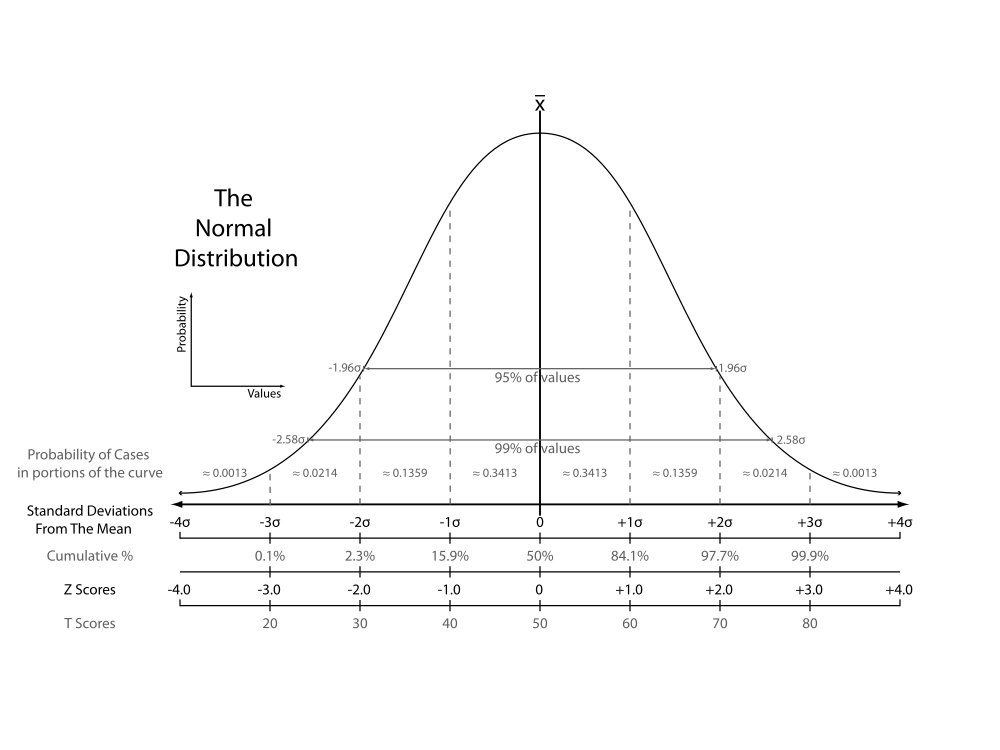
Returning to our 100-flip test statistics, we can see "how normal" they are:
test_stat_zscores = (test_stats_500 - test_stats_500.mean()) / test_stats_500.std()
plt.hist(test_stat_zscores)
plt.show()

def print_std_dev_props(zscores):
    # Within 1 std dev
    for i in range(1,4):
        prop_within = len([ts for ts in zscores if (ts <= i) and (ts >= -i)]) / len(zscores)
        print(f"% within {i} standard deviations: {prop_within * 100}")
print_std_dev_props(test_stat_zscores)
Not always the case! Recall our alternative test stat (test stat B):
test_stat_zscores_b = (test_stats_b - test_stats_b.mean()) / test_stats_b.std()
plt.hist(test_stat_zscores_b)
plt.show()

print_std_dev_props(test_stat_zscores_b)
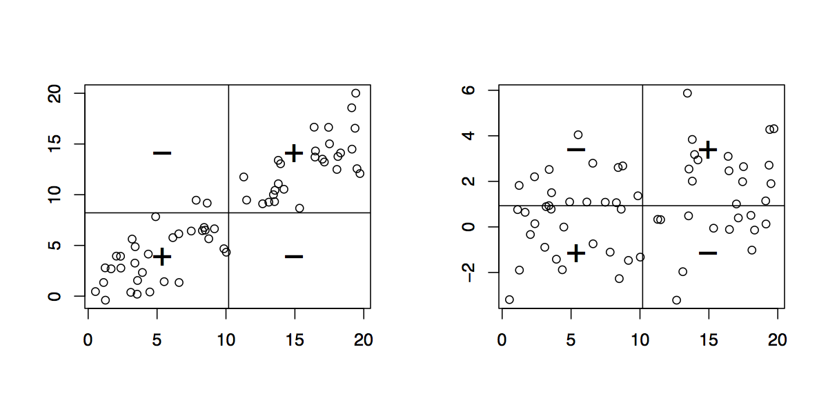
Correlation