Week 6: Adaptive Pooling in Multilevel Models, Bayesian Workflow
DSAN 5650: Causal Inference for Computational Social Science
Summer 2026, Georgetown University
Wednesday, June 24, 2026
Bayesian Workflow Seed-Planting
(Terms in HW2 we haven’t looked at yet!)

- Prior: Distribution over parameter values before seeing data
- Prior Predictive: Distribution over outcomes, before seeing data
- Posterior: Distribution over parameters, after seeing data
- Posterior Predictive: Distribution over outcomes, after seeing data
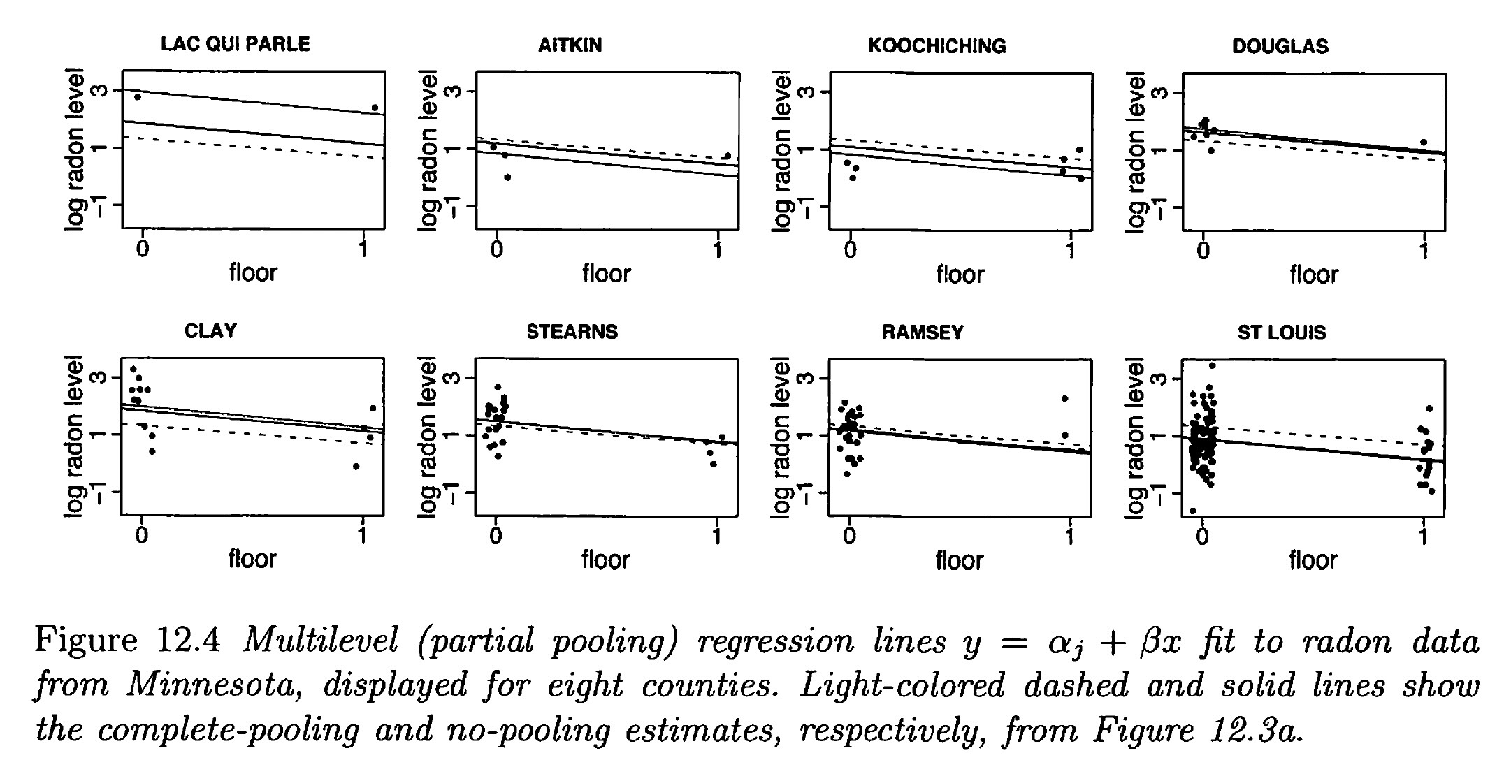
Pooling: None, Full, and Adaptive
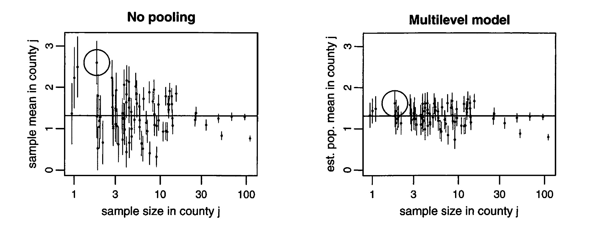
From Gelman and Hill (2007)
\[ \hat{\alpha}_j^{\text {multilevel }} = \frac{\frac{n_j}{\sigma_y^2} \bar{y}_j+\frac{1}{\sigma_\alpha^2} \bar{y}_{\text {all }}}{\frac{n_j}{\sigma_y^2}+\frac{1}{\sigma_\alpha^2}} \]
Why Adaptive >> None or Full?
\[ \alpha_j \sim \mathcal{N}(\mu_\alpha, \sigma_\alpha), \text{ for }j = 1, \ldots, J \]
- In the limit of \(\sigma_\alpha \rightarrow \infty\), the soft constraints do nothing, and there is no pooling;
- As \(\sigma_\alpha \rightarrow 0\), they pull the estimates all the way to zero, yielding the complete-pooling estimate
Bayesian Workflow
- Prior: Distribution over parameter values before seeing data
- Prior Predictive: Distribution over outcomes, before seeing data
- Posterior: Distribution over parameters, after seeing data
- Posterior Predictive: Distribution over outcomes, after seeing data
Modeling How Trees Become Forests
- Your model, if it’s generative (which… nearly all in 5650 are), relates observed data \(\mathbf{D}\) to a set of underlying parameters \(\boldsymbol{\theta}\) that are hypothesized as “giving rise” to \(\mathbf{D}\)
- When you specify how exactly this “giving rise” works, you’re specifying a DGP!
- PGMs: human-brain-friendly (bc graphical) language for writing DGPs; then move to PyAgrum \(\rightarrow\) Stan \(\rightarrow\) PyMC to “encode” PGMs (in
0100101) so computer can…
| Super-charge your EDA/modeling | Estimate \(\boldsymbol{\theta}\) from data |
|---|---|
| \(\leadsto\) Prior distributions | \(\leadsto\) Posterior distributions |
Code
library(tidyverse)
library(ggExtra)
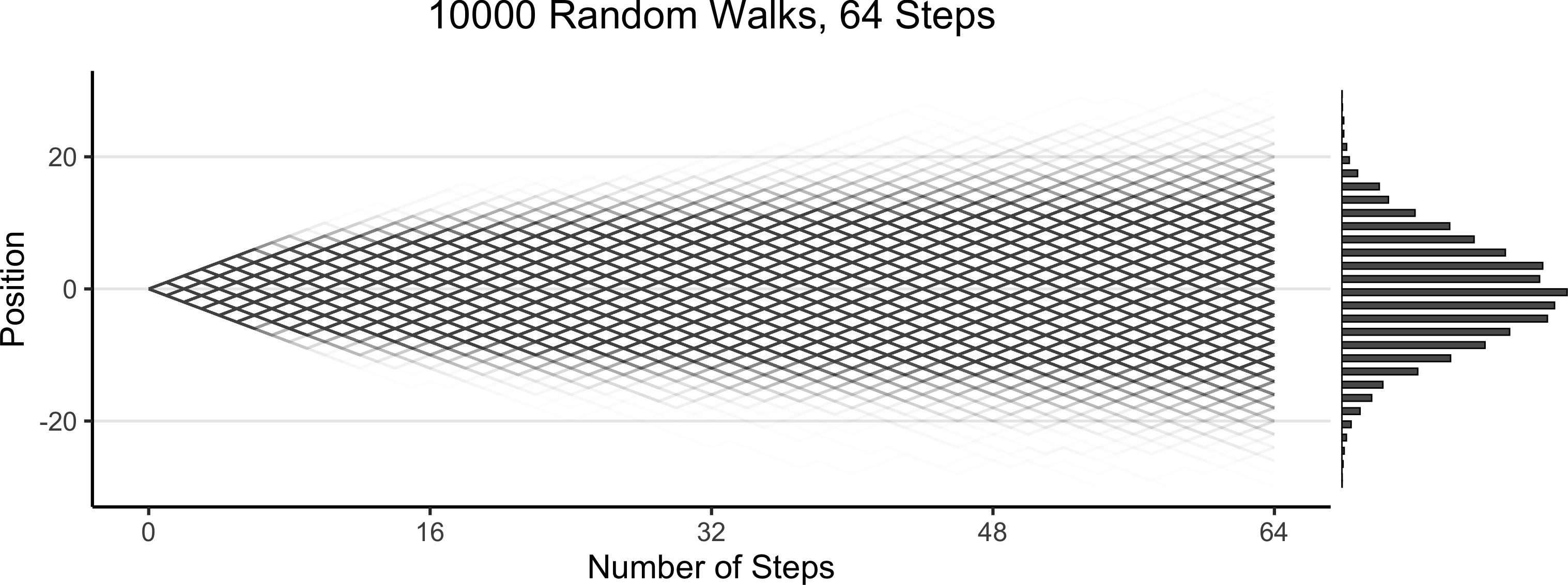
gen_walk_plot <- function(walk_data, a=0.0075) {
# print(end_df)
grid_color <- rgb(0, 0, 0, 0.1)
# And plot!
walkplot <- ggplot() +
geom_line(
data = walk_data$long_df,
aes(x = t, y = pos, group = pid),
linewidth = g_linewidth,
alpha = a,
#color = cb_palette[2]
#color = "#cf8f00"
color = "black"
) +
geom_point(
data = walk_data$end_df,
aes(x = t, y = endpos),
alpha = 0
) +
scale_x_continuous(
breaks = seq(
0,
walk_data$num_steps,
walk_data$num_steps / 4
)
) +
scale_y_continuous(
breaks = seq(-20, 20, 10)
) +
theme_dsan(base_size=24) +
theme(
legend.position = "none",
# title = element_text(size = 16)
) +
theme(
panel.grid.major.y = element_line(
color = grid_color,
linewidth = 1,
linetype = 1
)
) +
labs(
title = paste0(
walk_data$num_people, " Random Walks, ",
walk_data$num_steps, " Steps"
),
x = "Number of Steps",
y = "Position"
)
}
walk_data <- readRDS("assets/walk_data.rds")
# 16 steps
# wp1 <- gen_walkplot(500, 16, 0.05)
# ggMarginal(wp1, margins = "y", type = "histogram", yparams = list(binwidth = 1))
wp <- gen_walk_plot(walk_data) + ylim(-30,30)
ggMarginal(
wp, margins = "y",
type = "histogram",
yparams = list(binwidth = 1)
)
Prior “Stage” Distributions
- RVs \(\boldsymbol\theta\) = params of your model, RVs \(\mathbf{X}\) = data \(\leadsto\) Generative model \(\pedge{\boldsymbol\theta}{\mathbf{X}}\)
- Enter Prior World (Before observing any data): Since we have priors over \(\boldsymbol\theta\) \(\leadsto\) we can sample values of \(\boldsymbol\theta\), then generate synthetic data on the basis of these values
Prior Distribution: \(\Pr(\boldsymbol{\theta}^{❓})\)
What can I guess about values of my parameters from background knowledge of the world? e.g.:
- Human heights can’t be negative
- Data collected at a bar \(\Rightarrow\) Age \(\geq\) 18, \(\Pr(\text{Age} = x)\) decreases as \(x\) goes above 30

Prior Predictive Distribution: \(\Pr(\mathbf{X}^{❓} \mid \boldsymbol{\theta}^{❓})\)
What could the outcomes look like if I ran my guesses through the DGP?

100 simulated heights, none are negative
1K sim bar-goers; 80% have this haircut \(\rightarrow\)

Posterior “Stage” Distributions
- RVs \(\boldsymbol\theta\) = params of your model, RVs \(\mathbf{X}\) = data \(\leadsto\) Generative model \(\pedge{\boldsymbol\theta}{\mathbf{X}}\)
Posterior Distribution: \(\Pr\left(\boldsymbol{\theta} \; \middle| \; \mathbf{X} = \ponode{\mathbf{X}}\right)\)
Now we observe data: \(\pnode{\mathbf{X}} \leadsto \ponode{\mathbf{X}}\), which means we can use Bayes’ Rule to infer distribution over \(\boldsymbol{\theta}\): what values are most likely to produce \(\ponode{\mathbf{X}}\)?
- 60% of observed bar-goers have that haircut \(\Rightarrow\) \(\boldsymbol{\theta}_{\text{post}} \approx \frac{0.6 + 0.8}{2} = 0.7\)
- Coin = \(\textsf{H}\) 4/5 times \(\Rightarrow\) \(\boldsymbol{\theta} = p = \frac{0.5 + 0.8}{2} = 0.65\)
- Coin = \(\textsf{H}\) 5/5 times \(\Rightarrow\) \(\boldsymbol{\theta} = p = \frac{0.5 + 1.0}{2} = 0.75\)

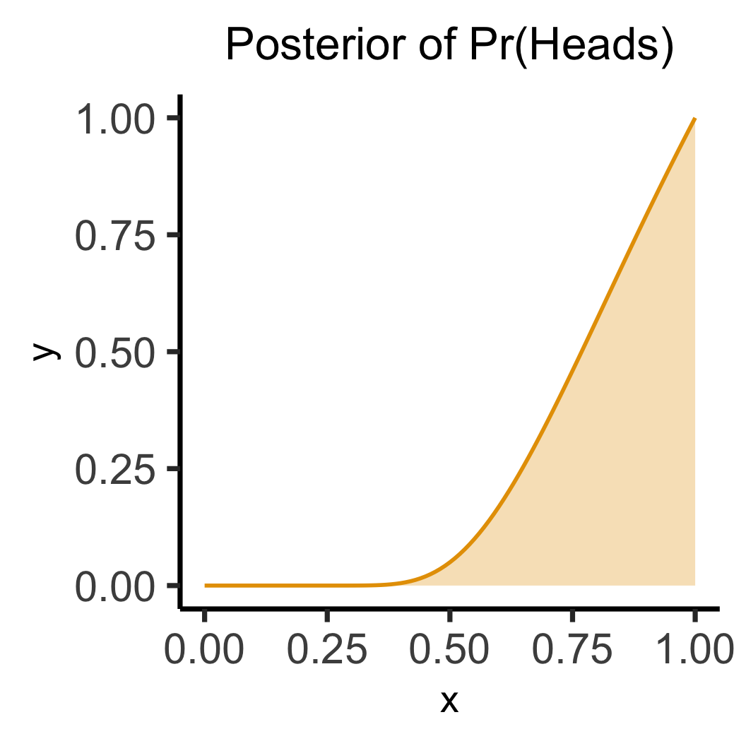
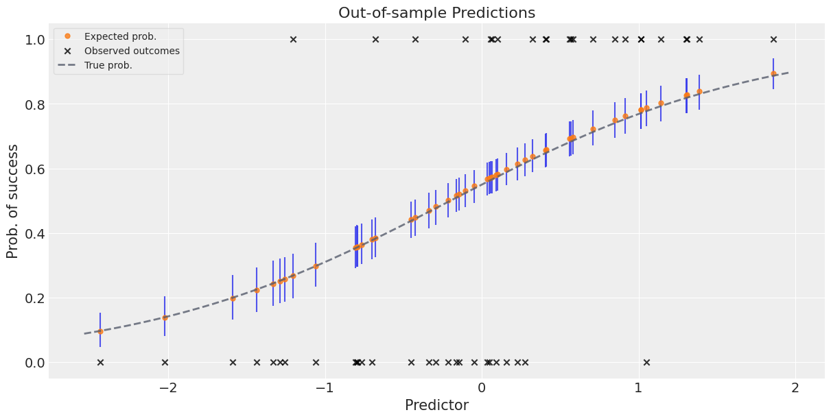
Posterior Predictive Distribution: \(\Pr(\mathbf{X} \mid \boldsymbol{\theta})\)
Now that we’ve fit \(\Pr(\boldsymbol{\theta})\) to data, can generate as much new data as we want, e.g. to evaluate how well model predicts outcomes for test data
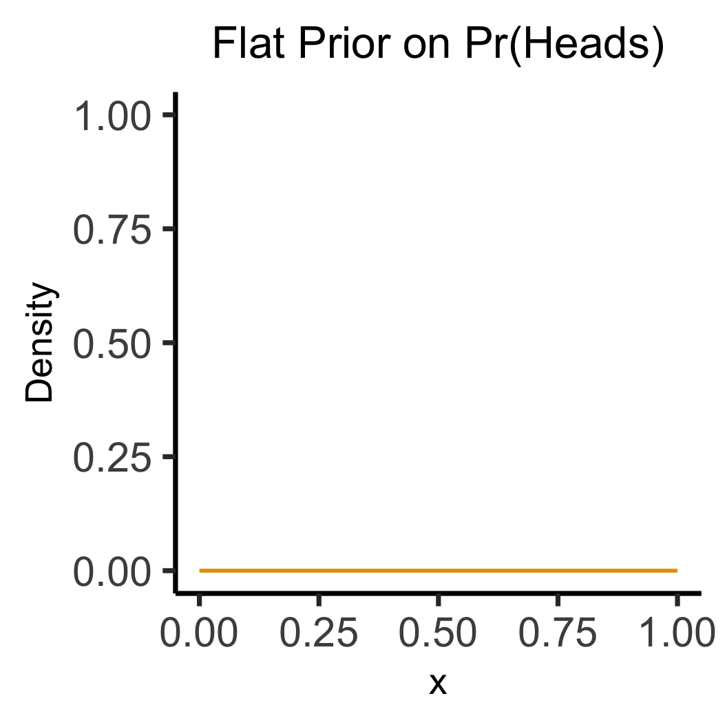
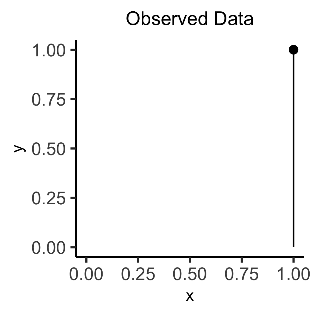
Flat vs. Informative Priors
Code
library(tidyverse)
flat_df <- tibble(x=seq(0, 1, 0.1), y=0)
flat_df |> ggplot(aes(x=x, y=y)) +
geom_line(
color=cb_palette[1],
linewidth=g_linewidth
) +
ylim(0, 1) +
labs(
title="Flat Prior on Pr(Heads)",
y="Density"
) +
theme_dsan(base_size=28) +
theme(title=element_text(size=20))
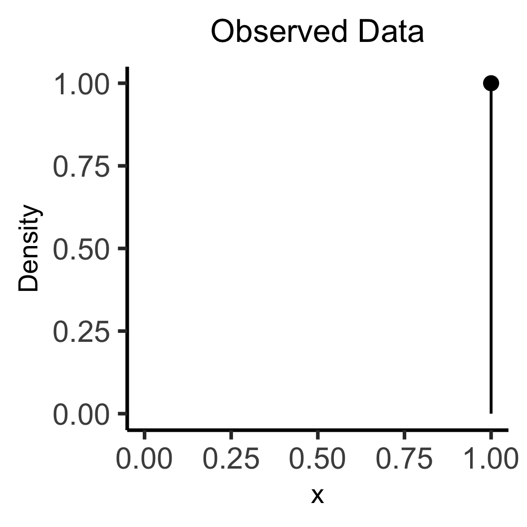
library(tidyverse)
data_df <- tibble(x=1, y=1)
data_df |> ggplot(aes(x=x, y=y)) +
geom_point(size=5) +
geom_segment(
x=1, y=0, yend=1, linewidth=g_linewidth
) +
xlim(0, 1) +
ylim(0, 1) +
labs(
title="Observed Data",
y="Density"
) +
theme_dsan(base_size=28) +
theme(title=element_text(size=20))
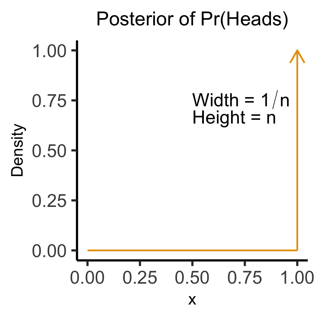
library(tidyverse)
library(latex2exp)
w_label <- TeX("Width = $1/n$")
h_label <- TeX("Height = $n$")
data_df <- tibble(x=1, y=1)
data_df |> ggplot(aes(x=x, y=y)) +
geom_segment(
x=1, y=0, yend=1, linewidth=g_linewidth,
color=cb_palette[1], arrow=arrow()
) +
geom_segment(
x=0, y=0, xend=1, linewidth=g_linewidth,
color=cb_palette[1]
) +
xlim(0, 1) +
ylim(0, 1) +
labs(
title="Posterior of Pr(Heads)",
y = "Density"
) +
theme_dsan(base_size=28) +
theme(title=element_text(size=20)) +
annotate(
geom = "text", x = 0.5, y = 0.8,
label = w_label, hjust = 0, vjust = 1, size = 8
) +
annotate(
geom = "text", x = 0.5, y = 0.7,
label = h_label, hjust = 0, vjust = 1, size = 8
)
\[ \otimes \]
\[ \leadsto \]
Code
library(tidyverse)
unif_df <- tibble(x=seq(0, 1, 0.1), y=1)
unif_df |> ggplot(aes(x=x, y=y)) +
  geom_line(
    color="#e69f00", linewidth=g_linewidth
  ) +
  annotate('rect', xmin=0, xmax=1, ymin=0, ymax=1, fill='#e69f00', alpha=0.3) +
  xlim(0, 1) + ylim(0, 1) +
  labs(title="Uniform Prior on Pr(Heads)") +
  theme_dsan(base_size=28) +
  theme(title=element_text(size=20))
library(tidyverse)
data_df <- tibble(x=1, y=1)
data_df |> ggplot(aes(x=x, y=y)) +
  geom_point(size=5) +
  geom_segment(
    x=1, y=0, yend=1, linewidth=g_linewidth
  ) +
  xlim(0, 1) +
  ylim(0, 1) +
  labs(title="Observed Data") +
  theme_dsan(base_size=28) +
  theme(title=element_text(size=20))
library(tidyverse)
data_df <- tibble(x=1, y=1)
x_vals <- seq(0, 1, 0.01)
my_exp <- function(x) exp(1-1/(x^2))
y_vals <- sapply(x_vals, my_exp)
data_df <- tibble(x=x_vals, y=y_vals)
rib_df <- tibble(x=x_vals, ymax=y_vals, ymin=0)
ggplot() +
  # stat_function(fun=my_exp, linewidth=g_linewidth, color=cb_palette[1]) +
  geom_line(
    data=data_df,
    aes(x=x, y=y),
    linewidth=g_linewidth, color=cb_palette[1]
  ) +
  geom_ribbon(
    data=rib_df,
    aes(x=x, ymin=ymin, ymax=ymax),
    fill=cb_palette[1], alpha=0.3
  ) +
  # geom_segment(
  #   x=1, y=0, yend=1, linewidth=g_linewidth,
  #   color=cb_palette[1], arrow=arrow()
  # ) +
  # geom_segment(
  #   x=0, y=0, xend=1, linewidth=g_linewidth,
  #   color=cb_palette[1]
  # ) +
  xlim(0, 1) +
  ylim(0, 1) +
  labs(title="Posterior of Pr(Heads)") +
  theme_dsan(base_size=28) +
  theme(title=element_text(size=20))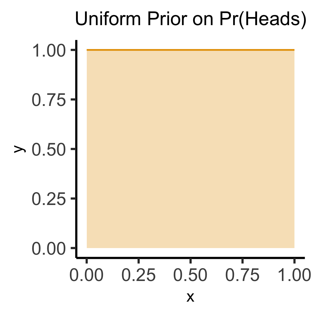
\[ \otimes \]
\[ \leadsto \]