Week 5: Multilevel Madness, Closing Backdoor Paths

DSAN 5650: Causal Inference for Computational Social Science
Summer 2026, Georgetown University

Jeff Jacobs

jj1088@georgetown.edu

Wednesday, June 17, 2026

Schedule

Today’s Planned Schedule:

	Start	End	Topic
Lecture	6:30pm	6:45pm	Reading Adventure 2, HW2 →
	6:45pm	7:30pm	The Logic of PGMs and Testable Hypotheses →
	6:45pm	7:30pm	Applying \(\textsf{do}()\) →
Break!	7:50pm	8:00pm
	8:00pm	9:00pm	Closing Backdoor Paths →

\[ \DeclareMathOperator*{\argmax}{argmax} \DeclareMathOperator*{\argmin}{argmin} \newcommand{\bigexp}[1]{\exp\mkern-4mu\left[ #1 \right]} \newcommand{\bigexpect}[1]{\mathbb{E}\mkern-4mu \left[ #1 \right]} \newcommand{\definedas}{\overset{\small\text{def}}{=}} \newcommand{\definedalign}{\overset{\phantom{\text{defn}}}{=}} \newcommand{\eqeventual}{\overset{\text{eventually}}{=}} \newcommand{\Err}{\text{Err}} \newcommand{\expect}[1]{\mathbb{E}[#1]} \newcommand{\expectsq}[1]{\mathbb{E}^2[#1]} \newcommand{\fw}[1]{\texttt{#1}} \newcommand{\given}{\mid} \newcommand{\green}[1]{\color{green}{#1}} \newcommand{\heads}{\outcome{heads}} \newcommand{\iid}{\overset{\text{\small{iid}}}{\sim}} \newcommand{\lik}{\mathcal{L}} \newcommand{\loglik}{\ell} \DeclareMathOperator*{\maximize}{maximize} \DeclareMathOperator*{\minimize}{minimize} \newcommand{\mle}{\textsf{ML}} \newcommand{\nimplies}{\;\not\!\!\!\!\implies} \newcommand{\orange}[1]{\color{orange}{#1}} \newcommand{\outcome}[1]{\textsf{#1}} \newcommand{\param}[1]{{\color{purple} #1}} \newcommand{\pgsamplespace}{\{\green{1},\green{2},\green{3},\purp{4},\purp{5},\purp{6}\}} \newcommand{\pedge}[2]{\require{enclose}\enclose{circle}{~{#1}~} \rightarrow \; \enclose{circle}{\kern.01em {#2}~\kern.01em}} \newcommand{\pnode}[1]{\require{enclose}\enclose{circle}{\kern.1em {#1} \kern.1em}} \newcommand{\ponode}[1]{\require{enclose}\enclose{box}[background=lightgray]{{#1}}} \newcommand{\pnodesp}[1]{\require{enclose}\enclose{circle}{~{#1}~}} \newcommand{\purp}[1]{\color{purple}{#1}} \newcommand{\sign}{\text{Sign}} \newcommand{\spacecap}{\; \cap \;} \newcommand{\spacewedge}{\; \wedge \;} \newcommand{\tails}{\outcome{tails}} \newcommand{\Var}[1]{\text{Var}[#1]} \newcommand{\bigVar}[1]{\text{Var}\mkern-4mu \left[ #1 \right]} \]

source("../dsan-globals/_globals.r")

library(tidyverse) # For ggplot
library(extraDistr) # For rbern()
library(patchwork) # For side-by-side plotting
library(ggtext) # For colors in titles
library(rethinking)
library(dagitty)
n_d <- 10000 # For discrete RVs
n_c <- 300 # For continuous RVs
source("mydrawdag.r")

Reading Adventure 2: Measuring Ideology / Polarization

congress_comb_df <- read_csv("assets/congress_means.csv") |>
  rename(Chamber = chamber)
gap_top <- 1.0 - max(congress_comb_df$party.mean.diff.d1)
plot_ymin <- min(congress_comb_df$party.mean.diff.d1) - gap_top
congress_comb_df |>
  ggplot(aes(x=year, y=party.mean.diff.d1, color=Chamber, alpha=Chamber)) +
  # geom_rect(
  #   aes(xmin = 1941, xmax = 1945, ymin = -Inf, ymax = 1.0),
  #   fill = "grey", alpha = 0.01, inherit.aes=FALSE,
  # ) +
  geom_rect(
    aes(xmin = 1929, xmax = 1939, ymin = -Inf, ymax = 1.0),
    fill = "grey", alpha = 0.01, inherit.aes=FALSE,
  ) +
  geom_text(
    aes(
      x=1929-1, y=0.4,
      label="Great\nDepression",
      hjust=1.0, vjust=0.0, lineheight=0.85
    ),
    inherit.aes=FALSE
  ) +
  geom_line() +
  geom_point() +
  theme_dsan(base_size=18) +
  ylim(plot_ymin, 1.0) +
  geom_hline(yintercept=1.0, linetype='dashed') +
  scale_x_continuous(breaks = seq(1880, 2025, by=20)) +
  scale_color_manual(
    values=c("Combined"="black", "House"="#e69f00", "Senate"="#56b4e9")
  ) +
  scale_alpha_manual(
    values=c("Combined"=0.9, "House"=0.45, "Senate"=0.45),
  ) +
  labs(
    title="Post Civil War Polarization (1879-2025)",
    x="Year",
    y="Difference in Party Mean Ideology",
  )

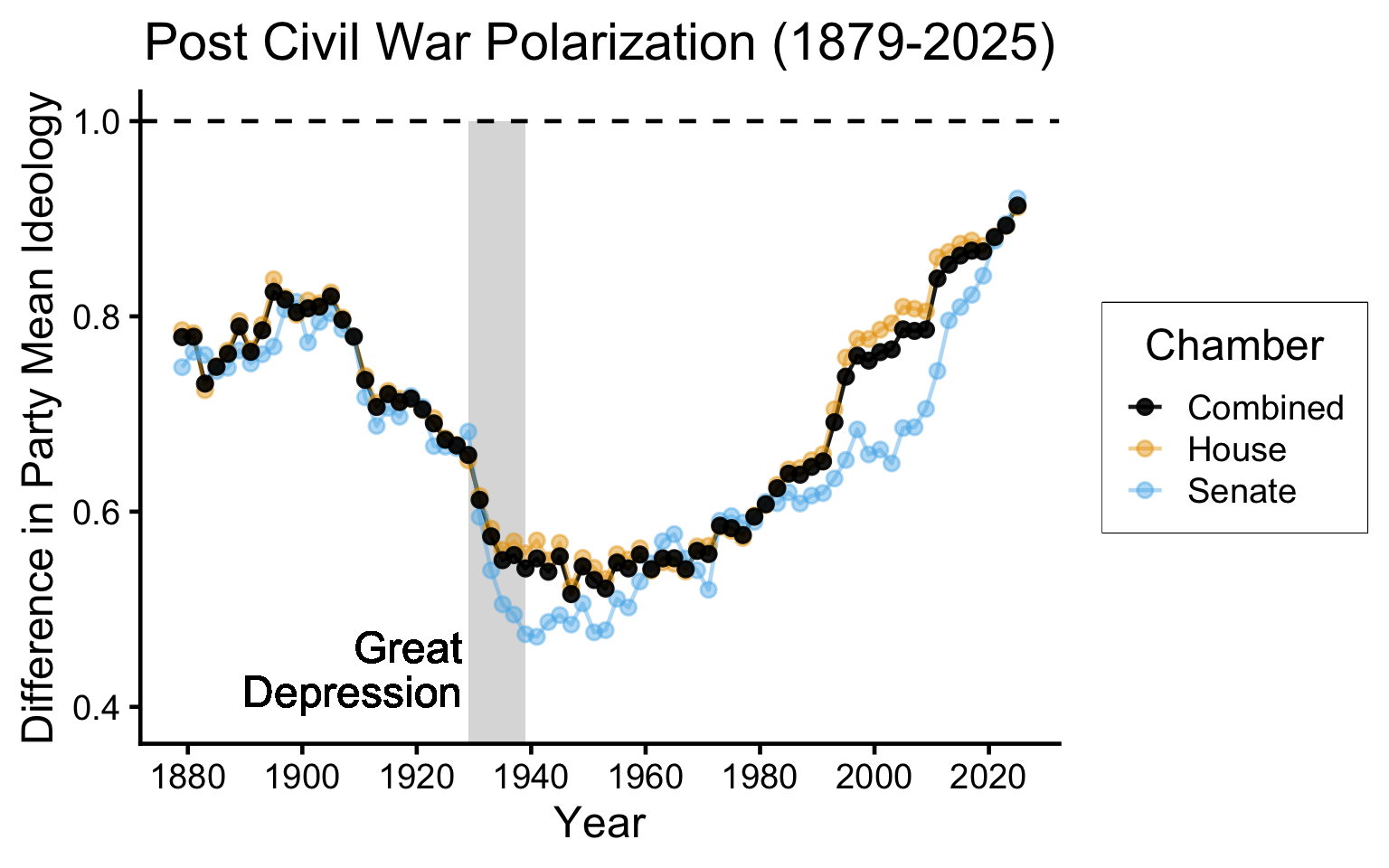
Figure 1: The “party gap” decreased from about 1900 until 1950, but has increased steadily since then

What Could Possibly Explain This?

gini_df <- read_csv("assets/mod_gini.csv")
mod_congress_df <- read_csv("assets/mod_congress.csv")
invert_rescale_gini <- function(scaled_vals, old_min, old_max, new_min, new_max) {
  old_min <- 0.348
  old_max <- 0.462
  new_min <- 0.5
  new_max <- 0.9
  inv_factor <- (scaled_vals - new_min) / (new_max - new_min)
  return(
    inv_factor * (old_max - old_min) + old_min
  )
}
ggplot() +
  # geom_rect(
  #   aes(xmin = 1941, xmax = 1945, ymin = -Inf, ymax = 1.0),
  #   fill = "grey", alpha = 0.01, inherit.aes=FALSE,
  # ) +
  geom_rect(
    aes(xmin = 1929, xmax = 1939, ymin = -Inf, ymax = Inf),
    fill = "grey", alpha = 0.01, inherit.aes=FALSE,
  ) +
  # geom_text(
  #   aes(
  #     x=1929-1, y=0.4,
  #     label="Great\nDepression",
  #     hjust=1.0, vjust=0.0, lineheight=0.85
  #   ),
  #   inherit.aes=FALSE
  # ) +
  geom_line(data=mod_congress_df, aes(x=year, y=value, color=name)) +
  geom_point(data=mod_congress_df, aes(x=year, y=value, color=name)) +
  geom_line(data=gini_df, aes(x=year, y=gini_scaled, color=name)) +
  geom_point(data=gini_df, aes(x=year, y=gini_scaled, color=name)) +
  theme_dsan(base_size=14) +
  scale_y_continuous(
    "Difference in Party Mean Ideology", 
    sec.axis = sec_axis(~ invert_rescale_gini(.), name = "Gini Coefficient")
  ) +
  labs(
    title="20th Century Inequality (1914-2025)",
    x="Year",
    y="Difference in Party Mean Ideology",
  ) +
  theme(legend.title = element_blank())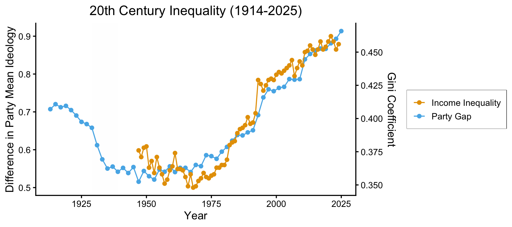

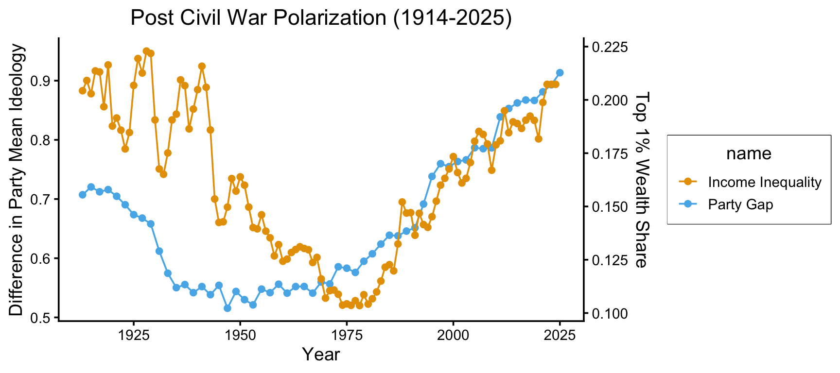
cong_gini_df <- inner_join(gini_df, mod_congress_df, by=join_by(year))
cor(cong_gini_df$value.x, cong_gini_df$value.y, use="complete.obs")

[1] 0.9671485

But Inequality \(\neq\) Wealth of Top 1%…

income_df <- read_csv("assets/income_ineq.csv")
invert_rescale_income <- function(scaled_vals, old_min, old_max, new_min, new_max) {
  old_min <- 0.1035
  old_max <- 0.2229
  new_min <- 0.52
  new_max <- 0.95
  inv_factor <- (scaled_vals - new_min) / (new_max - new_min)
  return(
    inv_factor * (old_max - old_min) + old_min
  )
}
ggplot() +
  # geom_rect(
  #   aes(xmin = 1941, xmax = 1945, ymin = -Inf, ymax = 1.0),
  #   fill = "grey", alpha = 0.01, inherit.aes=FALSE,
  # ) +
  geom_rect(
    aes(xmin = 1929, xmax = 1939, ymin = -Inf, ymax = Inf),
    fill = "grey", alpha = 0.01, inherit.aes=FALSE,
  ) +
  # geom_text(
  #   aes(
  #     x=1929-1, y=0.4,
  #     label="Great\nDepression",
  #     hjust=1.0, vjust=0.0, lineheight=0.85
  #   ),
  #   inherit.aes=FALSE
  # ) +
  geom_line(data=mod_congress_df, aes(x=year, y=value, color=name)) +
  geom_point(data=mod_congress_df, aes(x=year, y=value, color=name)) +
  geom_line(data=income_df, aes(x=year, y=value, color=name)) +
  geom_point(data=income_df, aes(x=year, y=value, color=name)) +
  theme_dsan(base_size=14) +
  scale_y_continuous(
    "Difference in Party Mean Ideology", 
    sec.axis = sec_axis(~ invert_rescale_income(.), name = "Top 1% Wealth Share")
  ) +
  labs(
    title="Post Civil War Polarization (1914-2025)",
    x="Year",
  )

cong_income_df <- inner_join(income_df, mod_congress_df, by=join_by(year))
cong_income_mod_df <- cong_income_df |> filter(year >= 1970)
cor(cong_income_mod_df$value.x, cong_income_mod_df$value.y, use="complete.obs")

[1] 0.9768329

HW2: Multilevel Madness

We will open and look at it today after the break!

The Four Elemental Confounds… Today: What to Do About Them!

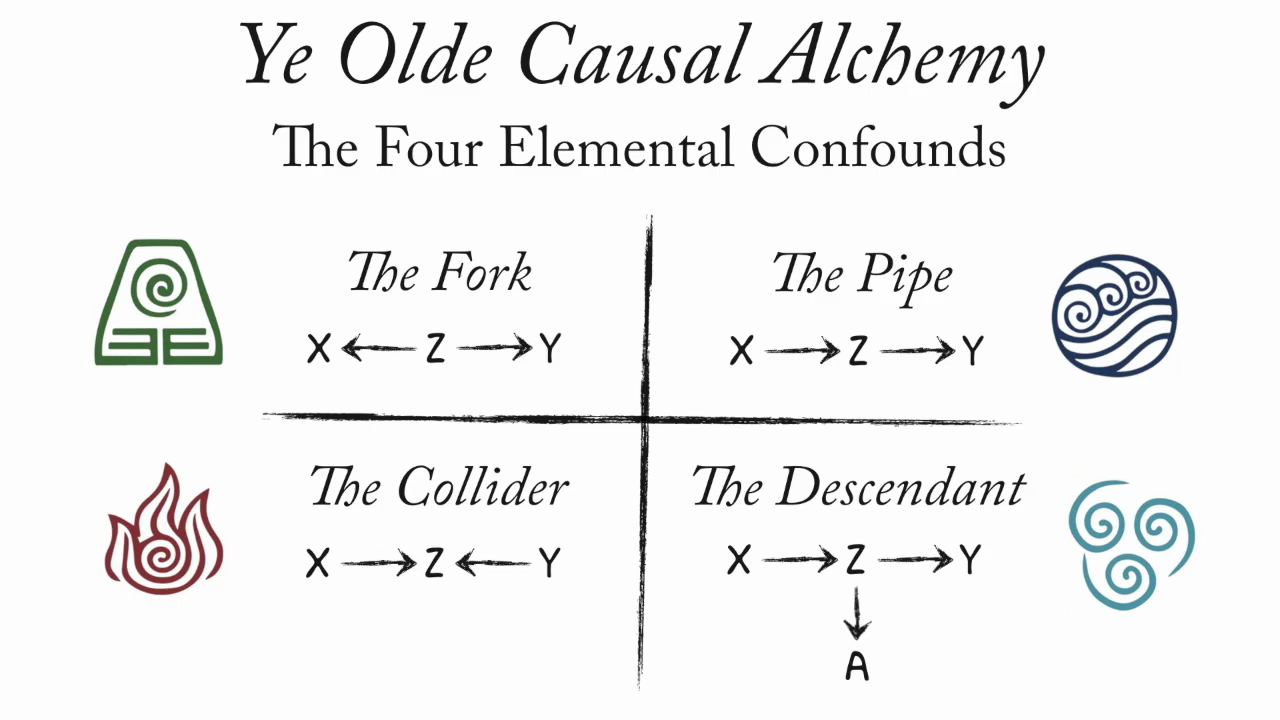
From Richard McElreath’s Statistical Rethinking Lectures

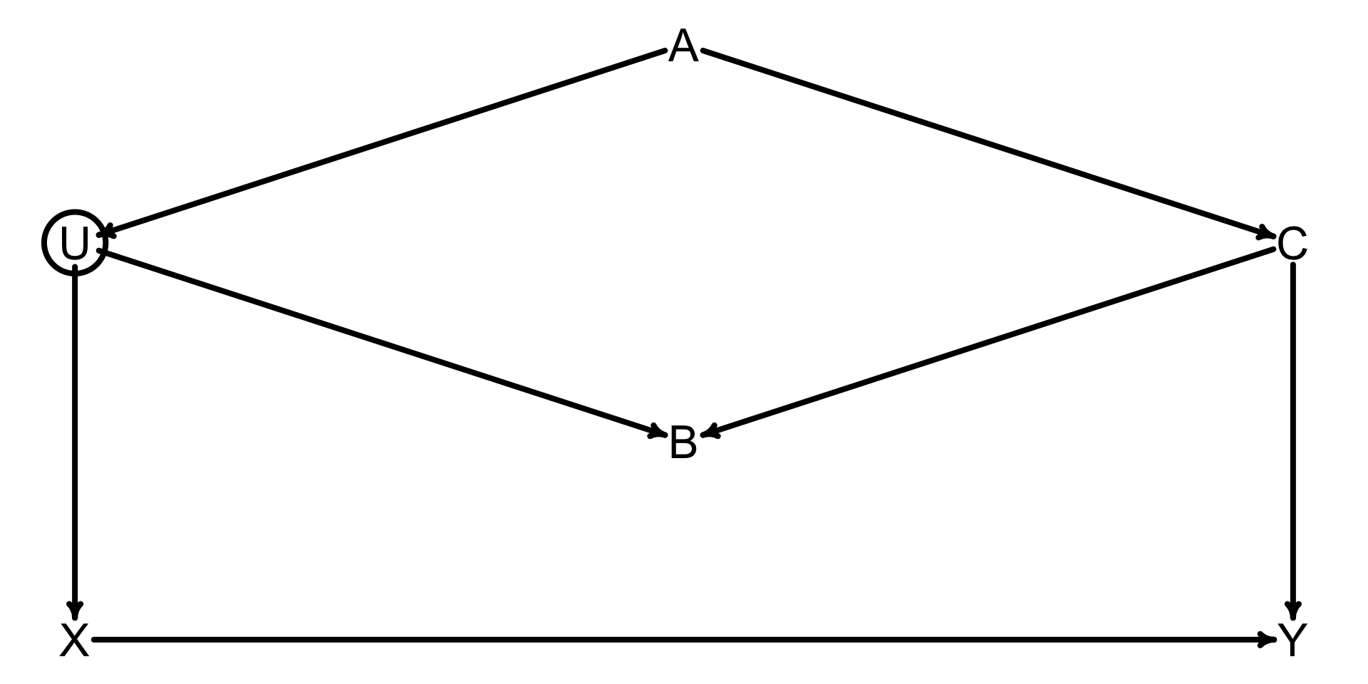
Blocking Backdoor Paths

dagitty: R interface to dagitty.net

rt_dag <- dagitty("dag{
X [exposure]
Y [outcome]
U [unobserved]
X -> Y
X <- U <- A -> C -> Y
U -> B <- C
}")
coordinates(rt_dag) <- list(
  x=c(U=0, X=0, A=0.5, B=0.5, C=1, Y=1),
  y=c(X=0.75, Y=0.75, B=0.5, U=0.25, C=0.25, A=0)
)
drawdag_jj(
  rt_dag, cex=2.5, lwd=3, radius=7, arr.width=0.6, arr.length=0.6, shift_arrows=FALSE
)

Two backdoor paths!

\(X \leftarrow \require{enclose}\enclose{circle}{U} \leftarrow A \rightarrow C \rightarrow Y\): Open or closed?

\(X \leftarrow \require{enclose}\enclose{circle}{U} \rightarrow B \leftarrow C \rightarrow Y\): Open or closed?

adjustmentSets(rt_dag)

{ C }
{ A }

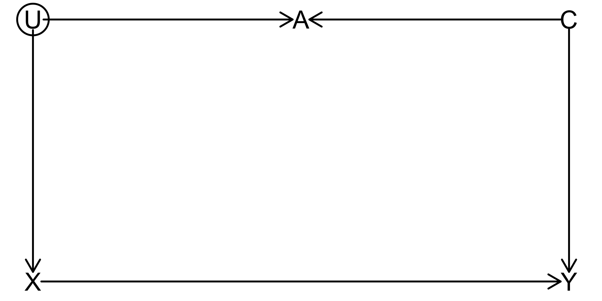
Collider Bias / Included Variable Bias

rt_dag <- dagitty("dag{
X [exposure]
Y [outcome]
U [unobserved]
X -> Y
X <- U
Y <- C
U -> A <- C
}")
coordinates(rt_dag) <- list(
  x=c(U=0, X=0, A=0.5, C=1, Y=1),
  y=c(X=0.75, Y=0.75, U=0.25, C=0.25, A=0.25)
)
drawdag_jj(
  rt_dag, cex=2.5, lwd=3, radius=7, arr.width=0.6, arr.length=0.6, shift_arrows=FALSE
)

Backdoor paths?

Adjustments needed?

Collider Bias / Included Variable Bias: Answers

rt_dag <- dagitty("dag{
X [exposure]
Y [outcome]
U [unobserved]
X -> Y
X <- U
Y <- C
U -> A <- C
}")
coordinates(rt_dag) <- list(
  x=c(U=0, X=0, A=0.5, C=1, Y=1),
  y=c(X=0.75, Y=0.75, U=0.25, C=0.25, A=0.25)
)
drawdag_jj(
  rt_dag, cex=2.5, lwd=3, radius=7, arr.width=0.6, arr.length=0.6, shift_arrows=FALSE
)

Backdoor paths?

\(X \leftarrow \require{enclose}\enclose{circle}{U} \rightarrow A \leftarrow C \rightarrow Y\): Closed

Adjustments needed?

adjustmentSets(rt_dag)

{}

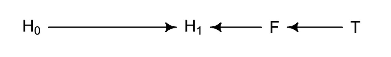
First “Real” Example: Anti-Fungal Soil Treatment

• \(H_0\): Height at time \(t = 0\)
• \(H_1\): Height at time \(t = 1\)
• \(F\): Fungus growth amount
• \(T\): Fungal treatment applied?

impliedConditionalIndependencies(plant_dag)

F _||_ H_0
H_0 _||_ T
H_1 _||_ T | F

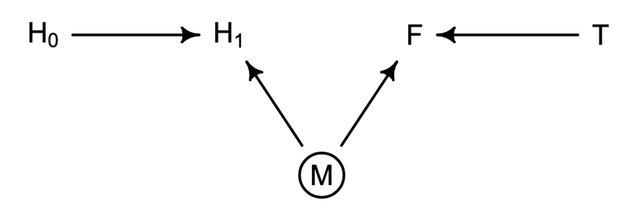
Alternative: Unobserved Moisture

• \(H_0\): Height at time \(t = 0\)
• \(H_1\): Height at time \(t = 1\)
• \(F\): Fungus growth amount
• \(T\): Fungal treatment applied?
• \(M\): Moisture level

References