Week 3: From PGMs to Causal Diagrams

DSAN 5650: Causal Inference for Computational Social Science
Summer 2026, Georgetown University

Jeff Jacobs

jj1088@georgetown.edu

Wednesday, June 3, 2026

Schedule

Today’s Planned Schedule:

	Start	End	Topic
Lecture	6:30pm	6:45pm	HW1 Questions and Concerns →
	6:45pm	7:15pm	Causality Recap →
	7:00pm	7:30pm	Motivating Examples: Causal Inference →
	7:30pm	7:45pm	Your First Probabilistic Graphical Model! →
Break!	7:45pm	8:00pm
	8:00pm	9:00pm	PGM “Lab” →

\[ \DeclareMathOperator*{\argmax}{argmax} \DeclareMathOperator*{\argmin}{argmin} \newcommand{\bigexp}[1]{\exp\mkern-4mu\left[ #1 \right]} \newcommand{\bigexpect}[1]{\mathbb{E}\mkern-4mu \left[ #1 \right]} \newcommand{\definedas}{\overset{\small\text{def}}{=}} \newcommand{\definedalign}{\overset{\phantom{\text{defn}}}{=}} \newcommand{\eqeventual}{\overset{\text{eventually}}{=}} \newcommand{\Err}{\text{Err}} \newcommand{\expect}[1]{\mathbb{E}[#1]} \newcommand{\expectsq}[1]{\mathbb{E}^2[#1]} \newcommand{\fw}[1]{\texttt{#1}} \newcommand{\given}{\mid} \newcommand{\green}[1]{\color{green}{#1}} \newcommand{\heads}{\outcome{heads}} \newcommand{\iid}{\overset{\text{\small{iid}}}{\sim}} \newcommand{\lik}{\mathcal{L}} \newcommand{\loglik}{\ell} \DeclareMathOperator*{\maximize}{maximize} \DeclareMathOperator*{\minimize}{minimize} \newcommand{\mle}{\textsf{ML}} \newcommand{\nimplies}{\;\not\!\!\!\!\implies} \newcommand{\orange}[1]{\color{orange}{#1}} \newcommand{\outcome}[1]{\textsf{#1}} \newcommand{\param}[1]{{\color{purple} #1}} \newcommand{\pgsamplespace}{\{\green{1},\green{2},\green{3},\purp{4},\purp{5},\purp{6}\}} \newcommand{\pedge}[2]{\require{enclose}\enclose{circle}{~{#1}~} \rightarrow \; \enclose{circle}{\kern.01em {#2}~\kern.01em}} \newcommand{\pnode}[1]{\require{enclose}\enclose{circle}{\kern.1em {#1} \kern.1em}} \newcommand{\ponode}[1]{\require{enclose}\enclose{box}[background=lightgray]{{#1}}} \newcommand{\pnodesp}[1]{\require{enclose}\enclose{circle}{~{#1}~}} \newcommand{\purp}[1]{\color{purple}{#1}} \newcommand{\sign}{\text{Sign}} \newcommand{\spacecap}{\; \cap \;} \newcommand{\spacewedge}{\; \wedge \;} \newcommand{\tails}{\outcome{tails}} \newcommand{\Var}[1]{\text{Var}[#1]} \newcommand{\bigVar}[1]{\text{Var}\mkern-4mu \left[ #1 \right]} \]

Logistics

🆕 JAH AutoHinter Documentation at jjacobs.me/jah  🆕

HW1 Questions / Concerns?

Labs + Reading Adventures coming this+next week:

Labs	Reading Quests
Lab 1: Novelty and Resonance in French Revolution Debates #InformationTheory#TextAnalysis	RQ 1: How to Do Things with Rhetoric #InformationTheory#TextAnalysis#WarsOfIdeas Corpora: (Elster 1996; Kassenova 2022; Schoenhals 1992; Mishal and Aharoni 1994; Oireachtas 2022) Style vs. Content: (Wang et al. 2017)
Lab 2: Optical Illusions as Causal Colliders #CausalGraphs#MindPlayinTricksOnMe#WebPPL	RQ 2: Hitler’s Willing Executioners? (Imai 2018) #EcologicalInference#PyMC
Lab 3: DW-NOMINATE, Latent Ideology, and Campaign Financing #LatentVariables	RQ 3: PGMs for Horowitz (1985), Ethnic Groups in Conflict #PGMs#Operationalization

W02 Recap: Aleatory vs. Epistemic Probability

• Social science, with “science” used in the same sense as for physics, may be a quixotic endeavor¹
• Instead, we’ll do social science, where we use data to…
• Infer tendencies: \(\mathsf{H}\) = «\(X\) tends to cause \(Y\)»
• With some degree of veracity: \(\Pr(\mathcal{H}) \approx 0.7\)
• Construct models that we can update with new evidence: Bayes’ rule! \(\Pr(\mathcal{H} \mid E) = \frac{\Pr(E \mid \mathcal{H} ) \Pr(\mathcal{H})}{\Pr(E)} \approx 0.8\)
• Notice “slippage” between aleatory probability within \(\mathcal{H}\) (“tends to”) vs. epistemic probability “outside of”, talking about \(\mathcal{H}\) (“I’m 70% confident about \(\mathcal{H}\)”)

1. At least, for the time being… BUT see Sperber (1996), which will come up later

Disclaimer: Unfortunate Side Effects of Engaging Seriously with Causality

You’ll no longer be able to read “scientific” writing without striking this expression (involuntarily):

“Scientific” talks will begin to sound like the following:

Blasting Off Into Causality!

Data-Generating Processes (DGPs)

• You saw this in DSAN 5100!
• «\(X_1, \ldots, X_n\) drawn i.i.d. Normal, mean \(\mu\) variance \(\sigma^2\)» characterizes DGP of \((X_1, \ldots, X_n)\)

• 5650: Dive into DGPs, rather than treating as black box/footnote to Law of Large Numbers, so we can move [asymptotically!]…
• From associational statements:
  «\(\underbrace{\text{An increase}}_{\small\text{noun}}\) in \(X\) by 1 is associated with increase in \(Y\) by \(\beta\)»
• To causal ones: «\(\underbrace{\text{Increasing}}_{\small\text{verb}}\) \(X\) by 1 causes \(Y\) to increase by \(\beta\)»

Causality in the Social World

• Thing we observe (poking out of water): data
• Hidden but possibly discoverable via deeper dive (ecosystem under surface): DGP
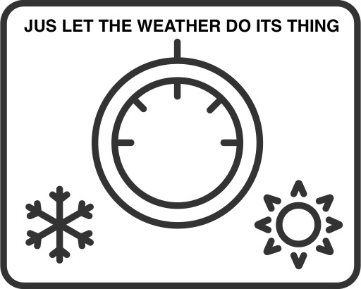
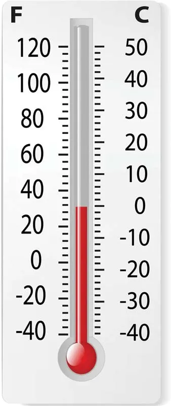
• Plz remember centrality of DGP! [Heat \(\rightarrow\) Thermometer Level]

Figure 1: Will putting Mr. Guns-Dog in timeout prevent plate-breaking?

potted_plant One Last Metaphor…

The \(\textsf{do}(\cdot)\) operator mutates DGPs!

Your First PGM!

From Probabilistic Models of Cognition, Ch 4

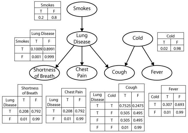
• Which of the variables (ovals) are observed? Which are latent?
• What do you think the arrows represent?
• Can we use this to find the “root cause” of (e.g.) observed chest pain? Or conversely, to predict possible ↑ in likelihood of chest pain if we start smoking?

Bayesian Inference but with Pictures

A Probabilistic Graphical Model (PGM) provides us with:

• A formal-mathematical…
• But also easily visualizable (by construction)…
• Representation of a data-generating process (DGP)!

Example: Let’s model how weather \(W\) affects evening plans \(Y\): the choice between going to a party or staying in to watch movies

DGP: The Partier’s Dilemma

1. A person \(i\) wakes up with some initial affinity for partying: \(\Pr(Y_i = \textsf{Go})\)
2. \(i\) then goes to their window and observes the weather \(W_i\) outside:
   1. If weather is sunny, \(i\)’s affinity increases: \(\Pr(Y_i = \textsf{Go} \mid W_i = \textsf{Sun}) > \Pr(Y = \textsf{Go})\)
   2. Otherwise, if rainy, \(i\)’s affinity decreases: \(\Pr(Y_i = \textsf{Go} \mid W_i = \textsf{Rain}) < \Pr(Y = \textsf{Go})\)

Two Main “Building Blocks”

Nodes like \(\require{enclose}\enclose{circle}{X}\) denote Random Variables:

\[ \require{enclose}\boxed{\enclose{circle}{X}} \simeq \boxed{ \begin{array}{c|cc}x & \textsf{Tails} & \textsf{Heads} \\\hline \Pr(X = x) & 0.5 & 0.5\end{array}} \]

Edges like \(\require{enclose}\enclose{circle}{X} \rightarrow \enclose{circle}{Y}\) denote relationships between RVs

• What an edge “means” can get [ontologically] tricky! (We’ll change the meaning when we move to causal PGMs)

• Retain sanity by just remembering: edge \(\require{enclose}\enclose{circle}{X} \rightarrow \enclose{circle}{Y}\) is included if we “care about” modeling conditional probability of \(Y\) given values of \(X\)

  \[ \require{enclose}\boxed{ \enclose{circle}{X} \rightarrow \enclose{circle}{Y} } \simeq \boxed{ \begin{array}{c|cc} x & \Pr(Y = \textsf{Lose} \mid X = x) & \Pr(Y = \textsf{Win} \mid X = x) \\\hline \textsf{Tails} & 0.8 & 0.2 \\ \textsf{Heads} & 0.5 & 0.5 \end{array} } \]

Full PGM Specification

• We have fully specified a PGM \(\mathcal{G}\) once we have provided:
  A list of nodes \(\{\require{enclose}\enclose{circle}{X_1}, \ldots, \enclose{circle}{X_n}\}\), one per RV \(X_i\)
  Conditional Probability Tables (CPTs) specifying \(\Pr(X_i \mid \text{Pa}(X_i))\) for all \(\require{enclose}\enclose{circle}{X_i}\)
• \(\text{Pa}(X_i)\) denotes all parents of \(X_i\) (sources of arrows pointing into \(\require{enclose}\enclose{circle}{X_i}\))

• Here \(\text{Pa}(\text{Cough}) = \{L, C\}\), so CPT for \(\text{Cough}\) provides \(\Pr(\text{Cough} = v \mid L = \ell, C = c)\) for all possible values \(v\) of \(\text{Cough}\), \(\ell\) of \(L\) (Lung Disease) and \(c\) of \(C\) (Cold)
• \(\text{Pa}(\text{Smokes}) = \varnothing\)! So CPT for \(\text{Smokes}\) only needs to provide \(\Pr(S = s)\) for the two possible values \(s \in \mathcal{R}_S = \{\textsf{F}, \textsf{T}\}\)

potted_plant Intervening…

 
Before…

\(\textsf{do}(G \leftarrow \textsf{A})\)

 
…After

PGM for the Partier’s Dilemma

• A node \(\require{enclose}\enclose{circle}{W}\) denoting RV \(W\), which can take on values in \(\mathcal{R}_W = \{\textsf{Sun}, \textsf{Rain}\}\),
• A node \(\require{enclose}\enclose{circle}{Y}\) denoting RV \(Y\), which can take on values in \(\mathcal{R}_Y = \{\textsf{Go}, \textsf{Stay}\}\), and
• An edge \(\require{enclose}\enclose{circle}{W} \rightarrow \enclose{circle}{Y}\) representing the following relationship between \(W\) and \(Y\):
  • \(\Pr(Y = \textsf{Go} \mid W = \textsf{Sun}) = 0.8\)
  • \(\Pr(Y = \textsf{Stay} \mid W = \textsf{Sun}) = 0.2\)
  • \(\Pr(Y = \textsf{Go} \mid W = \textsf{Rain}) = 0.1\)
  • \(\Pr(Y = \textsf{Stay} \mid W = \textsf{Rain}) = 0.9\)

Figure 2: Our PGM of the Partier’s Dilemma

	\(\Pr(Y = \textsf{Stay} \mid W)\)	\(\Pr(Y = \textsf{Go} \mid W)\)
\(W = \textsf{Sun}\)	0.2	0.8
\(W = \textsf{Rain}\)	0.9	0.1

Figure 3: The Conditional Probability Table (CPT) for the edge \(\require{enclose}\enclose{circle}{W} \rightarrow \enclose{circle}{Y}\) in Figure 2

Observed vs. Latent Nodes

• PGMs help us make valid (Bayesian) inferences about the world in the face of incomplete information!
• \(\Rightarrow\) Two types of nodes based on available information:
  • Observed nodes (shaded)
  • Latent nodes (unshaded)
• \(\leadsto\) Can use our PGM as a weather-inference machine!
• If we observe \(i\) at a party, what can we infer about the weather outside [even if we can’t go outside and observe it]?

Observed Partier, Latent Weather

• We can draw this situation as a PGM with shaded and unshaded nodes, distinguishing what we know from what we’d like to infer:

❓

✅

• And we can now use Bayes’ Rule to compute how observed information (\(i\) at party \(\Rightarrow [Y = \textsf{Go}]\)) “flows” back into \(W\)

Computation via Bayes’ Rule

• Bayes’ Rule, \(\Pr(A \mid B) = \frac{\Pr(B \mid A)\Pr(A)}{\Pr(B)}\), tells us how to use info about \(\Pr(B \mid A)\) to obtain info about \(\Pr(A \mid B)\)!
• We use it to obtain a distribution for \(W\) updated to incorporate new info \([Y = \textsf{Go}]\):

\[ \begin{align*} &\Pr(W = \textsf{Sun} \mid Y = \textsf{Go}) = \frac{\Pr(Y = \textsf{Go} \mid W = \textsf{Sun}) \Pr(W = \textsf{Sun})}{\Pr(Y = \textsf{Go})} \\ =\, &\frac{\Pr(Y = \textsf{Go} \mid W = \textsf{Sun}) \Pr(W = \textsf{Sun})}{\Pr(Y = \textsf{Go} \mid W = \textsf{Sun}) \Pr(W = \textsf{Sun}) + \Pr(Y = \textsf{Go} \mid W = \textsf{Rain}) \Pr(W = \textsf{Rain})} \end{align*} \]

• Plug in info from CPT to obtain our new (conditional) probability of interest:

\[ \begin{align*} \Pr(W = \textsf{Sun} \mid Y = \textsf{Go}) &= \frac{(0.8)(0.5)}{(0.8)(0.5) + (0.1)(0.5)} = \frac{0.4}{0.4 + 0.05} \approx 0.89 \end{align*} \]

• We’ve learned something interesting! Observing \(i\) at the party \(\leadsto\) probability of sun jumps from \(0.5\) (“prior” estimate of \(W\), best guess without any other relevant info) to \(0.89\) (“posterior” estimate of \(W\), best guess after incorporating relevant info).

Importance of Observed vs. Latent Distinction!

• Across many different fields, hidden stumbling-block in your project may be failure to model this distinction and pursue its implications!

Figure 4: Your model failing to achieve its goal bc you haven’t yet distinguished observed vs. latent variables

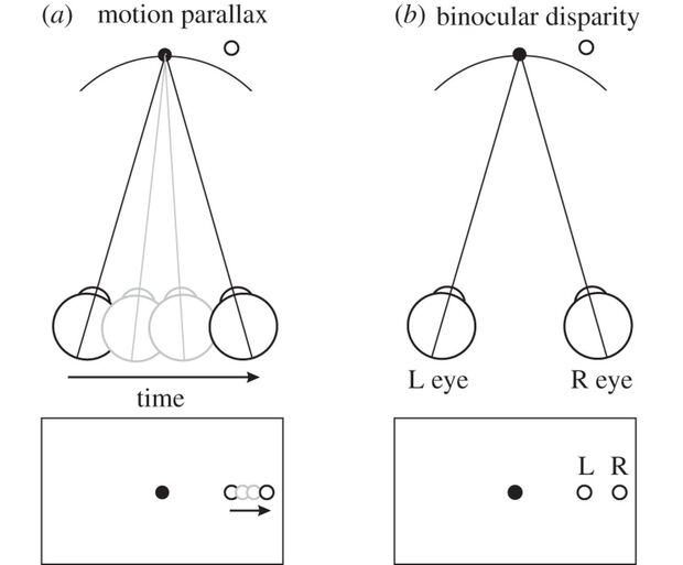
Example from Cognitive Neuroscience: Visual Perception

• We “see” 3D objects like a basketballs, but our eyes are (curved) 2D surfaces!
• \(\Rightarrow\) Our brains construct 3D environment by combining 2D info (observed photons-hitting-light-cones) with latent heuristic info:
  • Instantaneous Binocular Disparity, fusing info from two slightly-offset eyes,
  • Short-term Motion Parallax: How does object shift over short temporal “windows” of movement?
  • Long-term mental models (orange-ish circle with this line pattern is usually a basketball, which is usually this big, etc.)

Image source (a very cool article!)

• Similar examples in many other fields \(\leadsto\) science is a strange waltz of general models vs. field-specific details, but there’s one model that is infinitely helpful imo…

Hidden Markov Models (HMMs) Are Our Ur-PGMs!

• Using “Ur” in the same sense as “America’s Ur-Choropleths”…
• HMMs are our “Ur-Models” for Computational Social Science specifically

• Let’s consider an extremely currently-popular strand of CSS research, and step through why (a) it may be harder than it initially seems, but (b) we can use HMMs to “organize”/manage/visualize the complexity!

As in, how America’s Ur-Choropleths are two visualizations you can keep at hand before launching into a specific nation-wide choropleth about a specific issue!

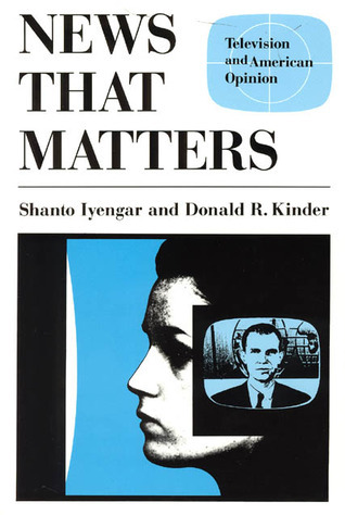
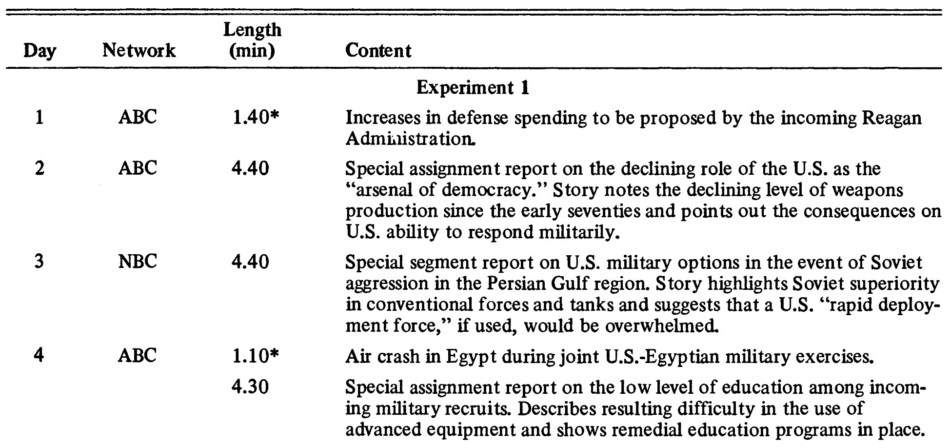
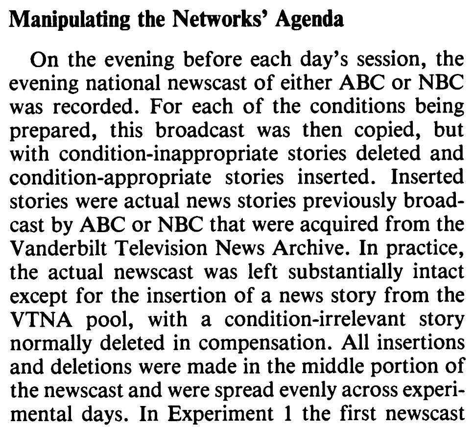
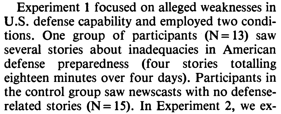
Studying “Fake News”

Studying “fake news” with ML and/or Deep Learning and/or Big Data is very popular in Computational Social Science: let’s use HMMs to see why it might be more… difficult/complicated than it seems at first 🙈

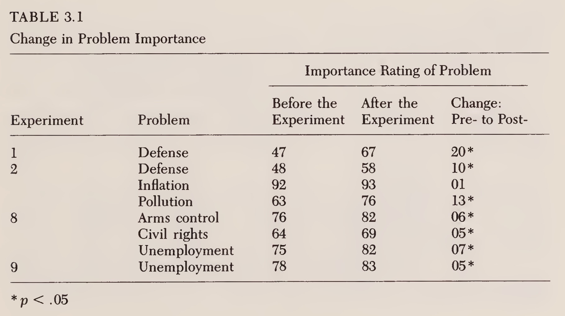
• The (implicit) model in studies like Iyengar and Kinder (2010) is something like:

• Thus allowing results to be summarized in a table like:

Iyengar and Kinder (2010)

The Devil in the Details I

Residents of the New Haven, Connecticut area participated in one of two experiments, each of which spanned six consecutive days […] took place in November 1980, shortly after the presidential election

We measured problem importance with four questions that appeared in both the pretreatment and posttreatment questionnaires:

• Please indicate how important you consider these problems to be.
• Should the federal government do more to develop solutions to these problems, even if it means raising taxes?
• How much do you yourself care about these problems?
• These days how much do you talk about these problems?

The Devil in the Details II

Randomization and Fine-Tuned Treatment

• …These are the types of things we usually don’t have control over as data scientists (we’re just handed a .csv!)

Let’s Model It!

The Final Piece: Plate Notation

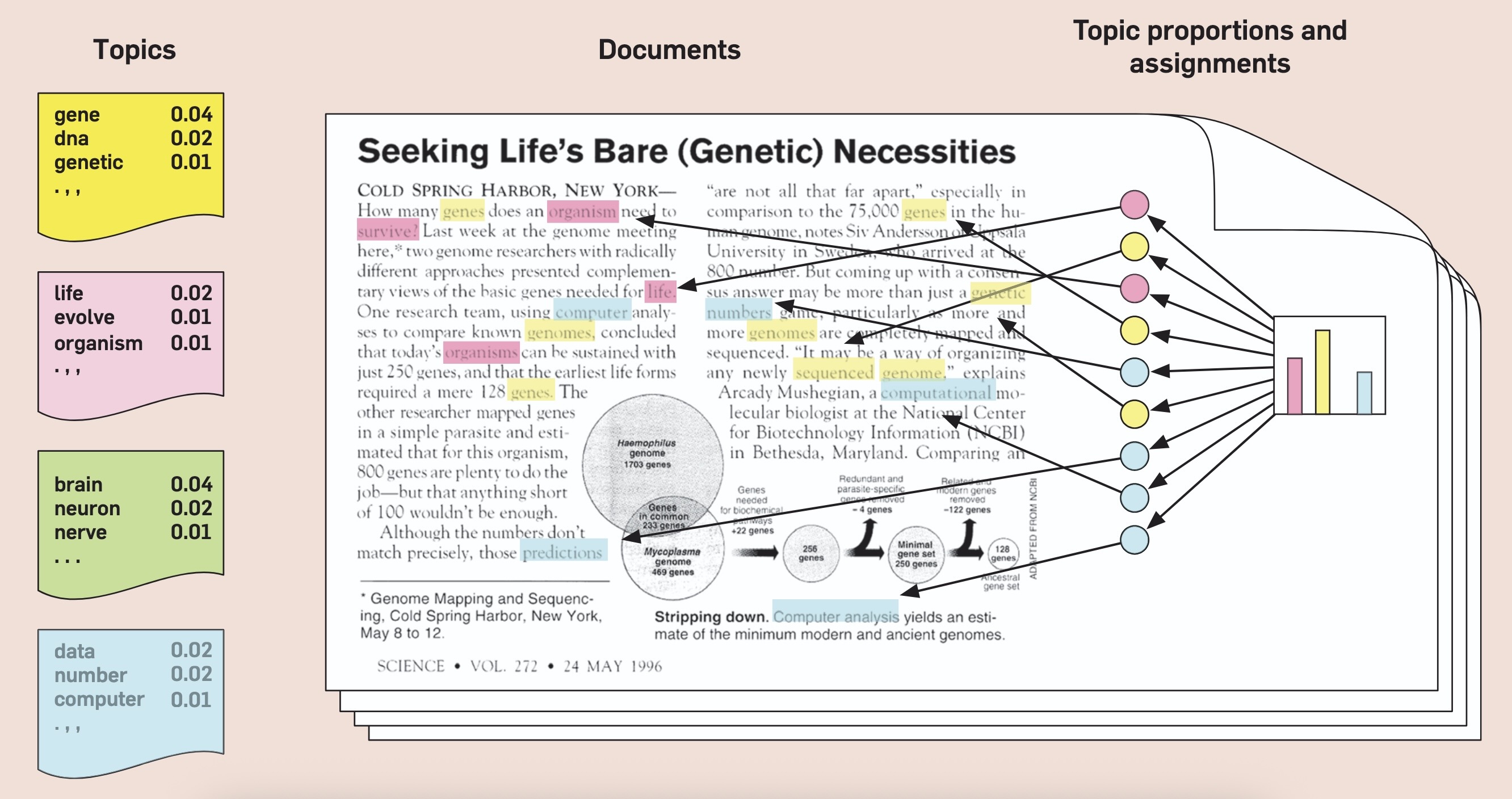
• For describing general distributions, there is often a “single node generating a bunch of nodes” structure:

• PGM notation has a built-in tool for this: plates!

Crucial CSS Model We Can Now Dive Into!

Image source

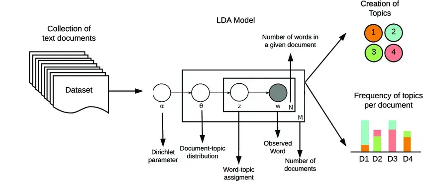
What Does This Give Us?

Before We Branch Off Of PGMs

(Even in non-causal settings)

Image source

• We don’t exactly think “Shakespeare decided on a set of topics, one per word-slot then chose a common word from each word slot”… and yet…!

Your First Causal Diagram

The Elite Hacker Known Only As GUMP

GUMP has figured out how to hack Georgetown grade servers, instantly zapping their grade up to an A+…

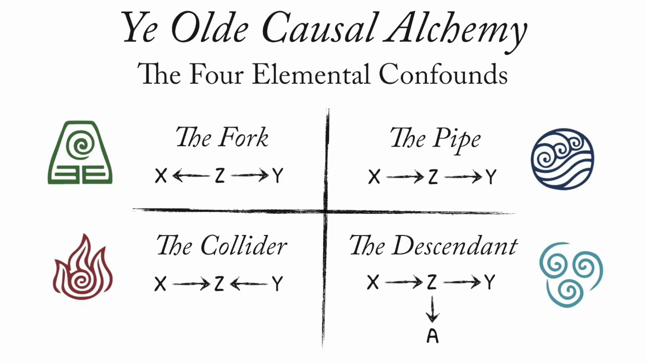
The Four Elemental Confounds

References

Barron, Alexander T. J., Jenny Huang, Rebecca L. Spang, and Simon DeDeo. 2018. “Individuals, Institutions, and Innovation in the Debates of the French Revolution.” Proceedings of the National Academy of Sciences 115 (18): 4607–12.

Blaydes, Lisa, Justin Grimmer, and Alison McQueen. 2018. “Mirrors for Princes and Sultans: Advice on the Art of Governance in the Medieval Christian and Islamic Worlds.” The Journal of Politics 80 (4): 1150–67.

Elster, Jon. 1996. The Roundtable Talks and the Breakdown of Communism. Chicago, IL: University of Chicago Press.

Horowitz, Donald L. 1985. Ethnic Groups in Conflict. University of California Press.

Imai, Kosuke. 2018. Quantitative Social Science: An Introduction. Princeton University Press.

Iyengar, Shanto, and Donald R. Kinder. 2010. News That Matters: Television & American Opinion. University of Chicago Press.

Kalyvas, Stathis N. 2006. The Logic of Violence in Civil War. Cambridge University Press.

Kassenova, Togzhan. 2022. Atomic Steppe: How Kazakhstan Gave Up the Bomb. Stanford, CA: Stanford University Press.

Koller, Daphne, and Nir Friedman. 2009. Probabilistic Graphical Models: Principles and Techniques. MIT Press.

Kozlowski, Austin C., Matt Taddy, and James A. Evans. 2019. “The Geometry of Culture: Analyzing the Meanings of Class Through Word Embeddings.” American Sociological Review 84 (5): 905–49.

Mishal, Shaul, and Reuben Aharoni. 1994. Speaking Stones: Communiqués from the Intifada Underground. Syracuse, NY: Syracuse University Press.

Oireachtas, Houses of the. 2022. “Explore the Treaty Debates – Houses of the Oireachtas.” Text. Houses of the Oireachtas. October 10, 2022.

Schoenhals, Michael. 1992. Doing Things with Words in Chinese Politics: Five Studies. Institute for East Asian Studies, University of California, Berkeley.

Sperber, Dan. 1996. Explaining Culture: A Naturalistic Approach. Cambridge: Blackwell.

Wang, Lu, Nick Beauchamp, Sarah Shugars, and Kechen Qin. 2017. “Winning on the Merits: The Joint Effects of Content and Style on Debate Outcomes.” Transactions of the Association for Computational Linguistics 5: 219–32.

Appendix 1: Zero Probabilities

From Koller and Friedman (2009), pp. 66-67:

Zero probabilities: A common mistake is to assign a probability of zero to an event that is extremely unlikely, but not impossible. The problem is that one can never condition away a zero probability, no matter how much evidence we get. When an event is unlikely but not impossible, giving it probability zero is guaranteed to lead to irrecoverable errors. For example, in one of the early versions of the the Pathfinder system (box 3.D), 10 percent of the misdiagnoses were due to zero probability estimates given by the expert to events that were unlikely but not impossible.

← Back to slide

Appendix 2: More Computational Social Science Examples

The Logic of Violence in Civil War

Kalyvas (2006)

Particularly Fun Non-“Standard” Examples

• Barron et al. (2018)
• Blaydes, Grimmer, and McQueen (2018)
• Kozlowski, Taddy, and Evans (2019)