Week 5: Tackling Overfitting with Cross-Validation
DSAN 5300: Statistical Learning
Spring 2026, Georgetown University
Monday, February 9, 2026
Our Working DGP
- Each country \(i\) has a certain \(x_i = \texttt{gdp\_per\_capita}_i\)
- They spend some portion of it on healthcare each year, which translates (based on the country’s healthcare system) into health outcomes \(y_i\)
- We operationalize these health outcomes as \(y_i = \texttt{DALY}_i\): Disability Adjusted Life Years, cross-nationally-standardized “lost years of minimally-healthy life”
Code
library(tidyverse) |> suppressPackageStartupMessages()
library(plotly) |> suppressPackageStartupMessages()
daly_df <- read_csv("assets/dalys_cleaned.csv")
daly_df <- daly_df |> mutate(
  gdp_pc_1k=gdp_pc_clean/1000
)
model_labels <- labs(
  x="GDP per capita ($1K PPP, 2021)",
  y="Log(DALYs/n)",
  title="Decrease in DALYs as GDP/n Increases"
)
daly_plot <- daly_df |> ggplot(aes(x=gdp_pc_1k, y=log_dalys_pc, label=name)) +
  geom_point() +
  # geom_smooth(method="loess", formula=y ~ x) +
  geom_smooth(method="lm", formula=y ~ poly(x,5), se=FALSE) +
  theme_dsan(base_size=14) +
  model_labels
ggplotly(daly_plot)
\[ \begin{align*} \leadsto Y = &10.58 - 0.2346 X + 0.01396 X^2 \\ &- 0.0004 X^3 + 0.000005 X^4 \\ &- 0.00000002 X^5 + \varepsilon \end{align*} \]
Code
eval_fitted_poly <- function(x) {
  coefs <- c(
    10.58,  -0.2346, 0.01396,
    -0.0004156, 0.0000053527, -0.0000000244
  )
  x_terms <- c(x^0, x^1, x^2, x^3, x^4, x^5)
  dot_prod <- sum(coefs * x_terms)
  return(dot_prod)
}
N <- 500
x_vals <- runif(N, min=0, max=90)
y_vals <- sapply(X=x_vals, FUN=eval_fitted_poly)
sim_df <- tibble(gdpc=x_vals, ldalys=y_vals)
ggplot() +
  geom_line(data=sim_df, aes(x=gdpc, y=ldalys)) +
  geom_point(data=daly_df, aes(x=gdp_pc_1k, y=log_dalys_pc)) +
  theme_dsan() +
  model_labels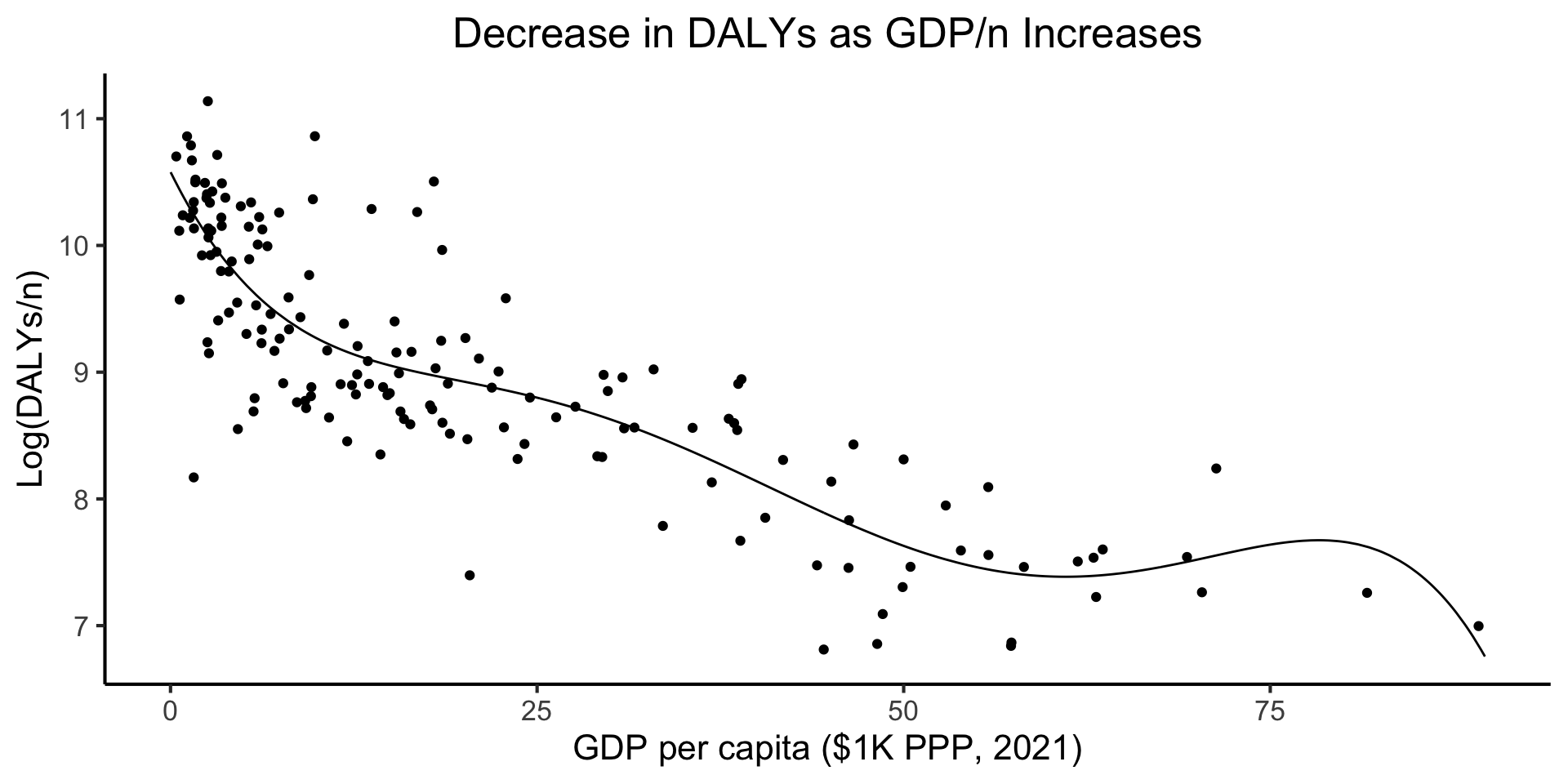
The “True” Model
- From here onwards, we adopt this as our “true” model, for pedagogical purposes!
- Meaning: we use this model to get a sense for how…
- CV can “foresee” test error \(\leadsto\) confidence in CV
- Regularization can penalize overly-complex models \(\leadsto\) confidence in LASSO
- In the real world we don’t know the DGP!
- \(\implies\) We build our confidence here, then take off the training wheels irl: use CV/Regularization in hopes they can help us “uncover” the unknown DGP
Code
run_dgp <- function(world_label="Sim", N=60, x_max=90) {
  x_vals <- runif(N, min=0, max=x_max)
  y_raw <- sapply(X=x_vals, FUN=eval_fitted_poly)
  y_noise <- rnorm(N, mean=0, sd=0.8)
  y_vals <- y_raw + y_noise
  sim_df <- tibble(
    gdpc=x_vals,
    ldalys=y_vals,
    world=world_label
  )
  return(sim_df)
}
df1 <- run_dgp("World 1")
df2 <- run_dgp("World 2")
df3 <- run_dgp("World 3")
dgp_df <- bind_rows(df1, df2, df3)
dgp_df |> ggplot(aes(x=gdpc, y=ldalys)) +
  geom_point(aes(color=world)) +
  facet_wrap(vars(world)) +
  theme_dsan(base_size=22) +
  remove_legend() +
  model_labels +
  labs(title="Three Possible Realizations of our DGP")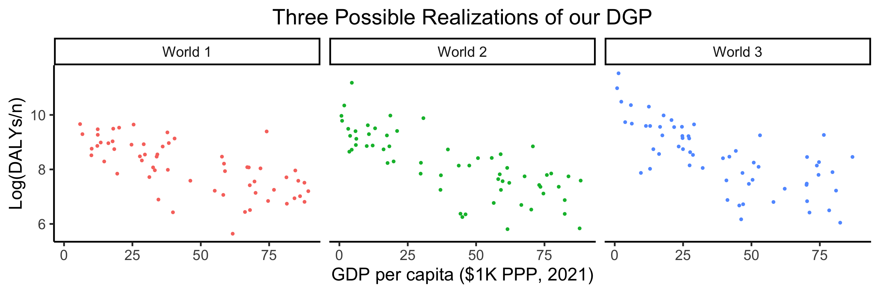
What We Have Thus Far
A core model, regression, that we can build up into p much anything we want!
| Class Topic | This Video |
|---|---|
| Linear regression | Pachelbel’s Canon in D (1m26s-1m46s) |
| Logistic regression | Add swing:  (1m46s) (1m46s) |
The Chilling Truth Behind Test Data 🫣
- Science-wise, technically, once you use the test set, you should stop working
- Full gory details in fancy books (Hume (1760) \(\rightarrow\) Popper (1934)), but the essence is captured by visualizing scientific inference (and statistical learning!) like:

- So, what do we do? Use \(\mathbf{D}_{\text{Tr}}\) along with knowledge of issues like overfitting to estimate test error!
- Fulfills our goal: find model which best predicts \(Y\) from \(X\) for unobserved data
How Does It Do for Our DGP?
- Recall that the “true” degree is 5, but that you’re not supposed to know that!
Code
library(boot)
set.seed(5300)
sim200_df <- run_dgp(
  world_label="N=200", N=200, x_max=100
)
sim1k_df <- run_dgp(
  world_label="N=1000", N=1000, x_max=100
)
compute_deltas <- function(df, min_deg=1, max_deg=12) {
  cv_deltas <- c()
  for (i in min_deg:max_deg) {
    cur_poly <- glm(ldalys ~ poly(gdpc, i), data=df)
    cur_poly_cv_result <- cv.glm(data=df, glmfit=cur_poly, K=5)
    cur_cv_adj <- cur_poly_cv_result$delta[1]
    cv_deltas <- c(cv_deltas, cur_cv_adj)
  }
  return(cv_deltas)
}
sim200_deltas <- compute_deltas(sim200_df)
sim200_delta_df <- tibble(degree=1:12, delta=sim200_deltas)
sim200_delta_df |> ggplot(aes(x=degree, y=delta)) +
  geom_line() +
  geom_point() +
  geom_vline(xintercept=5, linetype="dashed") +
  scale_x_continuous(
    breaks=seq(from=1,to=12,by=1)
  ) +
  theme_dsan(base_size=22) +
  labs(title="N = 200")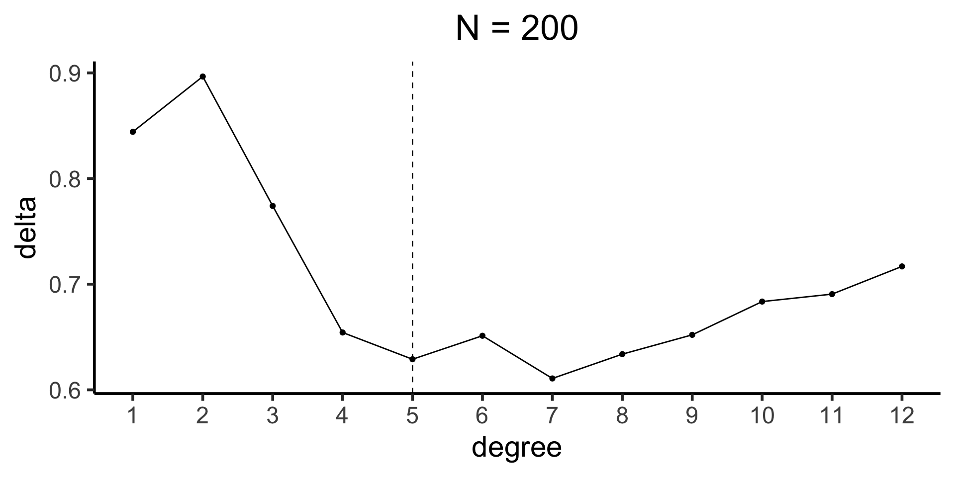
- Possible resolution: [See coming slides!]
Code
sim1k_deltas <- compute_deltas(sim1k_df)
sim1k_delta_df <- tibble(degree=1:12, delta=sim1k_deltas)
sim1k_delta_df |> ggplot(aes(x=degree, y=delta)) +
  geom_line() +
  geom_point() +
  geom_vline(xintercept=5, linetype="dashed") +
  scale_x_continuous(
    breaks=seq(from=1,to=12,by=1)
  ) +
  theme_dsan(base_size=22) +
  labs(title="N = 1000")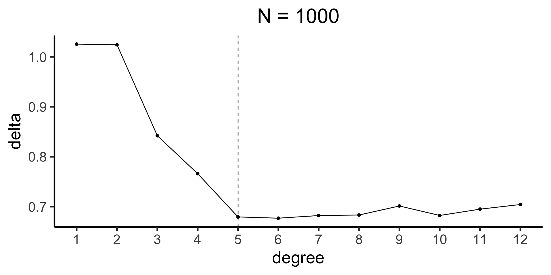
- Possible resolution: “one standard error rule”
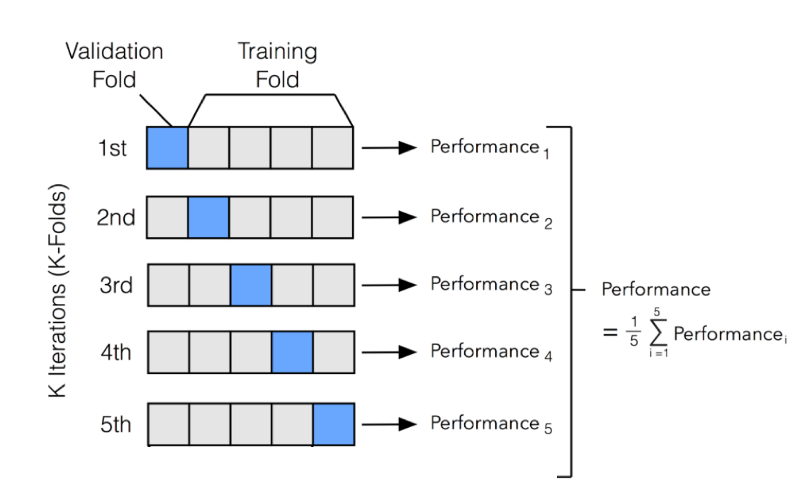
5-Fold Cross-Validation
- Secretly, by choosing a 20% fold to be the validation set earlier, I was priming you for 5-fold cross-validation!