Week 8: Support Vector Machines
DSAN 5300: Statistical Learning
Spring 2025, Georgetown University
Monday, March 10, 2025
Learning Decision Boundaries
- How can we get our computer to “learn” which houses I like?
Code
library(tidyverse) |> suppressPackageStartupMessages()
house_df <- tibble::tribble(
  ~sqm, ~yrs, ~Rating,
  10, 5, "Disliked",
  10, 20, "Disliked",
  20, 22, "Liked",
  25, 12, "Liked",
  11, 15, "Disliked",
  22.1, 5, "Liked"
) |> mutate(
  label = ifelse(Rating == "Liked", 1, -1)
)
base_plot <- house_df |> ggplot(aes(x=sqm, y=yrs)) +
  labs(
    title = "Jeff's House Search",
    x = "Square Meters",
    y = "Years Old"
  ) +
  expand_limits(x=c(0,25), y=c(0,25)) +
  coord_equal() +
  # 45 is minus sign, 95 is em-dash
  scale_shape_manual(values=c(95, 43)) +
  theme_dsan(base_size=14)
base_plot +
  geom_point(
    aes(color=Rating, shape=Rating), size=g_pointsize * 0.9,
    stroke=6
  ) +
  geom_point(aes(fill=Rating), color='black', shape=21, size=6, stroke=0.75, alpha=0.333)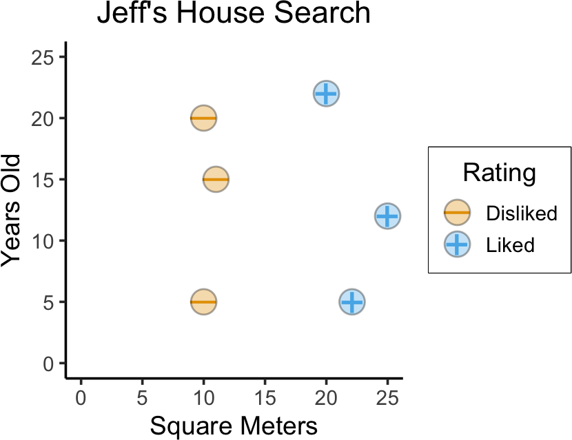
- Naïve idea: Try random lines (each forming a decision boundary), pick “best” one
Code
set.seed(5300)
is_separating <- function(beta_vec) {
  beta_str <- paste0(beta_vec, collapse=",")
  # print(paste0("is_separating: ",beta_str))
  margins <- c()
  for (i in 1:nrow(house_df)) {
    cur_data <- house_df[i,]
    # print(cur_data)
    linear_comb <- beta_vec[1] + beta_vec[2] * cur_data$sqm + beta_vec[3] * cur_data$yrs
    cur_margin <- cur_data$label * linear_comb
    # print(cur_margin)
    margins <- c(margins, cur_margin)
  }
  #print(margins)
  return(all(margins > 0) | all(margins < 0))
}
cust_rand_lines_df <- tribble(
  ~b0, ~b1, ~b2,
  # 41, -0.025, -1,
  165, -8, -1,
  -980, 62, -1
) |> mutate(
  slope=-(b1/b2),
  intercept=-(b0/b2)
)
num_lines <- 20
rand_b0 <- runif(num_lines, min=-40, max=40)
rand_b1 <- runif(num_lines, min=-2, max=2)
# rand_b2 <- -1 + 2*rbernoulli(num_lines)
rand_b2 <- -1
rand_lines_df <- tibble::tibble(
  id=1:num_lines,
  b0=rand_b0,
  b1=rand_b1,
  b2=rand_b2
) |> mutate(
  slope=-(b1/b2),
  intercept=-(b0/b2)
)
rand_lines_df <- bind_rows(rand_lines_df, cust_rand_lines_df)
# Old school for loop
for (i in 1:nrow(rand_lines_df)) {
  cur_line <- rand_lines_df[i,]
  cur_beta_vec <- c(cur_line$b0, cur_line$b1, cur_line$b2)
  cur_is_sep <- is_separating(cur_beta_vec)
  rand_lines_df[i, "is_sep"] <- cur_is_sep
}
base_plot +
  geom_abline(
    data=rand_lines_df, aes(slope=slope, intercept=intercept), linetype="dashed"
  ) +
  geom_point(
    aes(color=Rating, shape=Rating), size=g_pointsize * 0.9,
    stroke=6
  ) +
  geom_point(aes(fill=Rating), color='black', shape=21, size=6, stroke=0.75, alpha=0.333) +
  labs(
    title = paste0("10 Boundary Guesses"),
    x = "Square Meters",
    y = "Years Old"
  )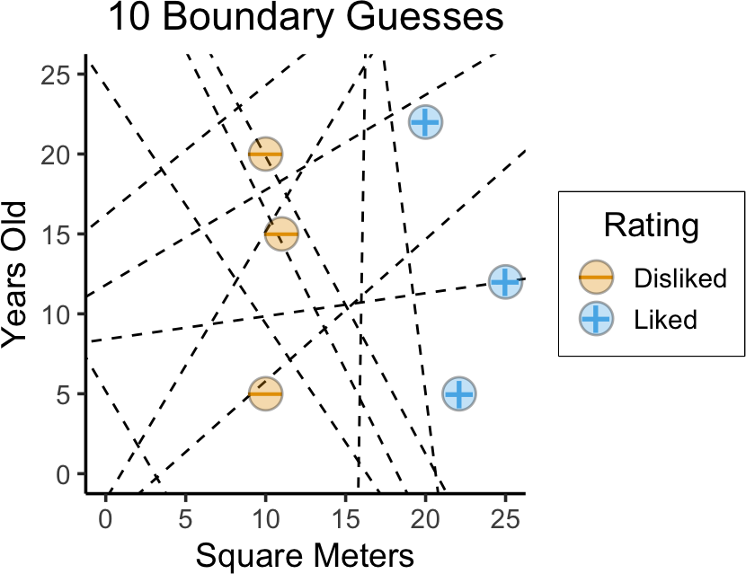
(…Which one is “best”?)
Separating Hyperplanes
- Any line which perfectly separates positive from negative cases is a separating hyperplane
Code
base_plot +
  geom_abline(
    data=rand_lines_df, aes(slope=slope, intercept=intercept, linetype=is_sep)
  ) +
  geom_abline(
    data=rand_lines_df |> filter(is_sep),
    aes(slope=slope, intercept=intercept),
    linewidth=3, color=cb_palette[4], alpha=0.333
  ) +
  scale_linetype_manual("Separating?", values=c("dotted", "dashed")) +
  geom_point(
    aes(color=Rating, shape=Rating), size=g_pointsize * 0.9,
    stroke=6
  ) +
  geom_point(aes(fill=Rating), color='black', shape=21, size=6, stroke=0.75, alpha=0.333) +
  labs(
    title = paste0("The Like vs. Dislike Boundary: 10 Guesses"),
    x = "Square Meters",
    y = "Years Old"
  )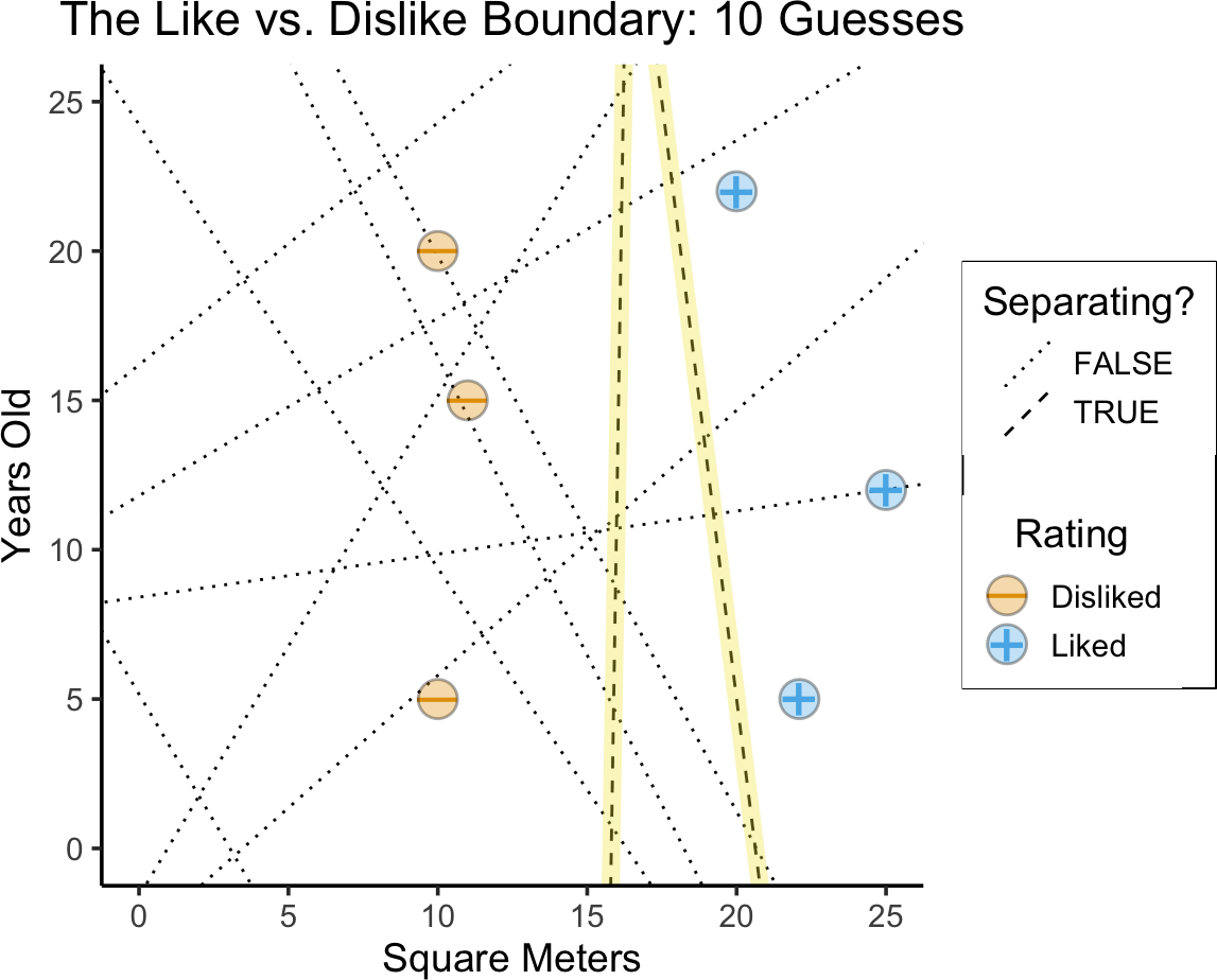
- Why might the left line be better? (Think of DGP!)
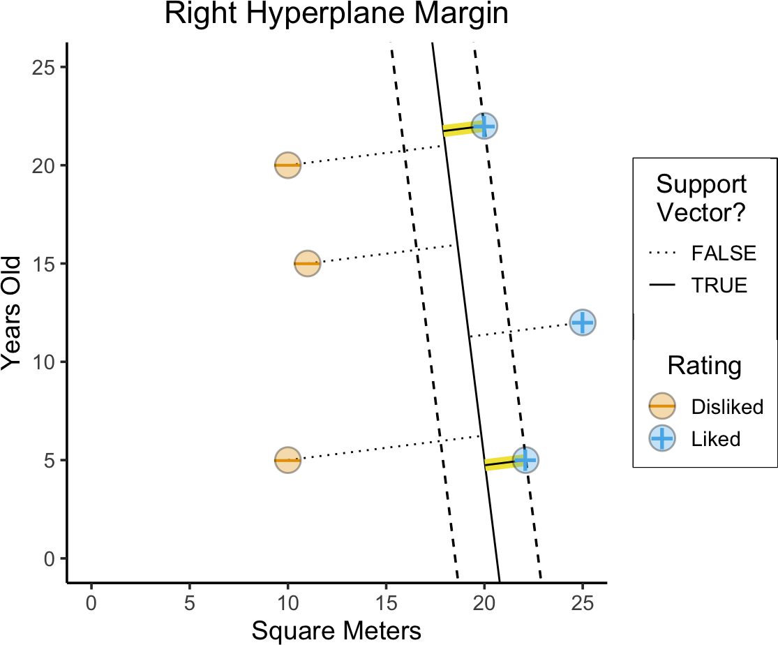
Max-Margin Hyperplanes
- Among the two, left hyperplane establishes a larger margin between the two classes!
- Margin (of hyperplane) = Smallest distance to datapoint (Think of hyperplane as middle of separating slab: how wide is the slab?)
- Important: Note how margin is not the same as average distance!
Code
sep_lines_df <- rand_lines_df |> filter(is_sep) |> mutate(
  norm_slope = (-1)/slope
)
cur_line_df <- sep_lines_df |> filter(slope > 0)
# left_line_df
# And make one copy per point
cur_sup_df <- uncount(cur_line_df, nrow(house_df))
cur_sup_df <- bind_cols(cur_sup_df, house_df)
cur_sup_df <- cur_sup_df |> mutate(
  norm_intercept = yrs - norm_slope * sqm,
  margin_intercept = yrs - slope * sqm,
  margin_intercept_gap = intercept - margin_intercept,
  margin_intercept_inv = intercept + margin_intercept_gap,
  norm_cross_x = -(norm_intercept - intercept) / (norm_slope - slope),
  x_gap = norm_cross_x - sqm,
  norm_cross_y = yrs + x_gap * norm_slope,
  vec_margin = label * (b0 + b1 * sqm + b2 * yrs),
  is_sv = vec_margin <= 240
)
base_plot +
  geom_abline(
    data=cur_line_df, aes(slope=slope, intercept=intercept), linetype="solid"
  ) +
  geom_abline(
    data=cur_sup_df |> filter(is_sv),
    aes(
      slope=slope,
      intercept=margin_intercept
    ),
    linetype="dashed"
  ) +
  geom_abline(
    data=cur_sup_df |> filter(is_sv),
    aes(
      slope=slope,
      intercept=margin_intercept_inv
    ),
    linetype="dashed"
  ) +
  geom_segment(
    data=cur_sup_df |> filter(is_sv),
    aes(x=sqm, y=yrs, xend=norm_cross_x, yend=norm_cross_y),
    color=cb_palette[4], linewidth=3
  ) +
  geom_segment(
    data=cur_sup_df,
    aes(x=sqm, y=yrs, xend=norm_cross_x, yend=norm_cross_y, linetype=is_sv)
  ) +
  geom_point(
    aes(color=Rating, shape=Rating), size=g_pointsize * 0.9,
    stroke=6
  ) +
  geom_point(aes(fill=Rating), color='black', shape=21, size=6, stroke=0.75, alpha=0.333) +
  scale_linetype_manual("Support\nVector?", values=c("dotted", "solid")) +
  labs(
    title = paste0("Left Hyperplane Distances"),
    x = "Square Meters",
    y = "Years Old"
  )
Code
# New calculation: line with same slope but that hits the SV
# y - y1 = m(x - x1), so...
# y - yrs = m(x - sqm) <=> y = m(x-sqm) + yrs <=> y = mx  - m*sqm + yrs
# <=> b = yrs - -m*sqm
cur_line_df <- sep_lines_df |> filter(slope < 0)
# left_line_df
# And make one copy per point
cur_sup_df <- uncount(cur_line_df, nrow(house_df))
cur_sup_df <- bind_cols(cur_sup_df, house_df)
cur_sup_df <- cur_sup_df |> mutate(
  norm_intercept = yrs - norm_slope * sqm,
  margin_intercept = yrs - slope * sqm,
  margin_intercept_gap = intercept - margin_intercept,
  margin_intercept_inv = intercept + margin_intercept_gap,
  norm_cross_x = -(norm_intercept - intercept) / (norm_slope - slope),
  x_gap = norm_cross_x - sqm,
  norm_cross_y = yrs + x_gap * norm_slope,
  vec_margin = abs(label * (b0 + b1 * sqm + b2 * yrs)),
  is_sv = vec_margin <= 25
)
base_plot +
  geom_abline(
    data=cur_line_df, aes(slope=slope, intercept=intercept), linetype="solid"
  ) +
  geom_abline(
    data=cur_sup_df |> filter(is_sv),
    aes(
      slope=slope,
      intercept=margin_intercept
    ),
    linetype="dashed"
  ) +
  geom_abline(
    data=cur_sup_df |> filter(is_sv),
    aes(
      slope=slope,
      intercept=margin_intercept_inv
    ),
    linetype="dashed"
  ) +
  # geom_abline(
  #   data=cur_line_df,
  #   aes(slope=slope, intercept=intercept),
  #   linewidth=3, color=cb_palette[4], alpha=0.333
  # ) +
  geom_segment(
    data=cur_sup_df |> filter(vec_margin <= 18),
    aes(x=sqm, y=yrs, xend=norm_cross_x, yend=norm_cross_y),
    color=cb_palette[4], linewidth=3
  ) +
  geom_segment(
    data=cur_sup_df,
    aes(x=sqm, y=yrs, xend=norm_cross_x, yend=norm_cross_y, linetype=is_sv)
  ) +
  geom_point(
    aes(color=Rating, shape=Rating), size=g_pointsize * 0.9,
    stroke=6
  ) +
  geom_point(aes(fill=Rating), color='black', shape=21, size=6, stroke=0.75, alpha=0.333) +
  scale_linetype_manual("Support\nVector?", values=c("dotted", "solid")) +
  labs(
    title = paste0("Right Hyperplane Margin"),
    x = "Square Meters",
    y = "Years Old"
  )
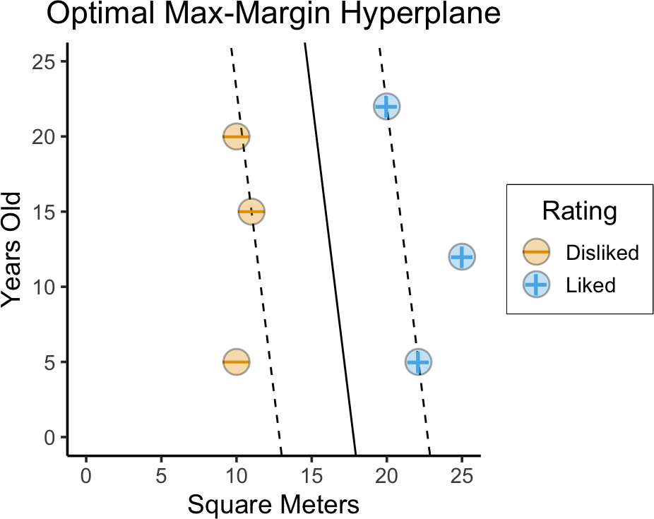
Optimal Max-Margin Hyperplane
- On previous slides we chose from a small set of randomly-generated lines…
- Now that we have max-margin objective, we can optimize over all possible lines!
- Any hyperplane can be written as \(\beta_0 + \beta_1 x_{1} + \beta_2 x_{2} = 0\)
Let \(y_i = \begin{cases} +1 &\text{if house }i\text{ Liked} \\ -1 &\text{if house }i\text{ Disliked}\end{cases}\)
\[ \begin{align*} \underset{\beta_0, \beta_1, \beta_2, M}{\text{maximize}}\text{ } & M \\ \text{s.t. } & y_i(\beta_0 + \beta_1 x_{i1} + \beta_2 x_{i2}) \geq M, \\ ~ & \beta_0^2 + \beta_1^2 + \beta_2^2 = 1 \end{align*} \]
- \(\beta_0^2 + \beta_1^2 + \beta_2^2 = 1\) just ensures that \(y_i(\beta_0 + \beta_1 x_{i1} + \beta_2 x_{i2})\) gives distance from hyperplane to \(x_i\)
Code
library(e1071)
liked <- as.factor(house_df$Rating == "Liked")
cent_df <- house_df
cent_df$sqm <- scale(cent_df$sqm)
cent_df$yrs <- scale(cent_df$yrs)
svm_model <- svm(liked ~ sqm + yrs, data=cent_df, kernel="linear")
cf <- coef(svm_model)
sep_intercept <- -cf[1] / cf[3]
sep_slope <- -cf[2] / cf[3]
# Invert Z-scores
sd_ratio <- sd(house_df$yrs) / sd(house_df$sqm)
inv_slope <- sd_ratio * sep_slope
inv_intercept <- mean(house_df$yrs) - inv_slope * mean(house_df$sqm) + sd(house_df$yrs)*sep_intercept
# And the margin boundary
sv_index <- svm_model$index[1]
sv_sqm <- house_df$sqm[sv_index]
sv_yrs <- house_df$yrs[sv_index]
margin_intercept <- sv_yrs - inv_slope * sv_sqm
margin_diff <- inv_intercept - margin_intercept
margin_intercept_inv <- inv_intercept + margin_diff
base_plot +
  coord_equal() +
  scale_shape_manual(values=c(95, 43)) +
  theme_dsan(base_size=14) +
  geom_abline(
    intercept=inv_intercept, slope=inv_slope, linetype="solid"
  ) +
  geom_abline(
    intercept=margin_intercept, slope=inv_slope, linetype="dashed"
  ) +
  geom_abline(
    intercept=margin_intercept_inv, slope=inv_slope, linetype="dashed"
  ) +
  geom_point(
    aes(color=Rating, shape=Rating), size=g_pointsize * 0.9,
    stroke=6
  ) +
  geom_point(aes(fill=Rating), color='black', shape=21, size=6, stroke=0.75, alpha=0.333) +
  scale_linetype_manual("Support\nVector?", values=c("dotted", "solid")) +
  labs(
    title = "Optimal Max-Margin Hyperplane",
    x = "Square Meters",
    y = "Years Old"
  )
When Does This Fail?
- What do we do in this case? (No separating hyperplane!)
Code
# Generate gaussian blob of disliked + gaussian
# blob of liked :3
library(mvtnorm) |> suppressPackageStartupMessages()
set.seed(5304)
num_houses <- 100
# Shared covariance matrix
Sigma_all <- matrix(c(12,0,0,20), nrow=2, ncol=2, byrow=TRUE)
# Negative datapoints
mu_neg <- c(10, 12.5)
neg_matrix <- rmvnorm(num_houses/2, mean=mu_neg, sigma=Sigma_all)
colnames(neg_matrix) <- c("sqm", "yrs")
neg_df <- as_tibble(neg_matrix) |> mutate(Rating="Disliked")
# Positive datapoints
mu_pos <- c(21, 12.5)
pos_matrix <- rmvnorm(num_houses/2, mean=mu_pos, sigma=Sigma_all)
colnames(pos_matrix) <- c("sqm", "yrs")
pos_df <- as_tibble(pos_matrix) |> mutate(Rating="Liked")
# And combine
nonsep_df <- bind_rows(neg_df, pos_df)
nonsep_df <- nonsep_df |> filter(yrs >= 5 & sqm <= 24 & sqm >= 7)
# Plot
nonsep_plot <- nonsep_df |> ggplot(aes(x=sqm, y=yrs)) +
  labs(
    title = "Jeff's House Search",
    x = "Square Meters",
    y = "Years Old"
  ) +
  # xlim(6,25) + ylim(2,22) +
  coord_equal() +
  # 45 is minus sign, 95 is em-dash
  scale_shape_manual(values=c(95, 43)) +
  theme_dsan(base_size=22)
nonsep_plot +
  geom_point(
    aes(color=Rating, shape=Rating), size=g_pointsize * 0.25,
    stroke=6
  ) +
  geom_point(aes(fill=Rating), color='black', shape=21, size=4, stroke=0.75, alpha=0.333)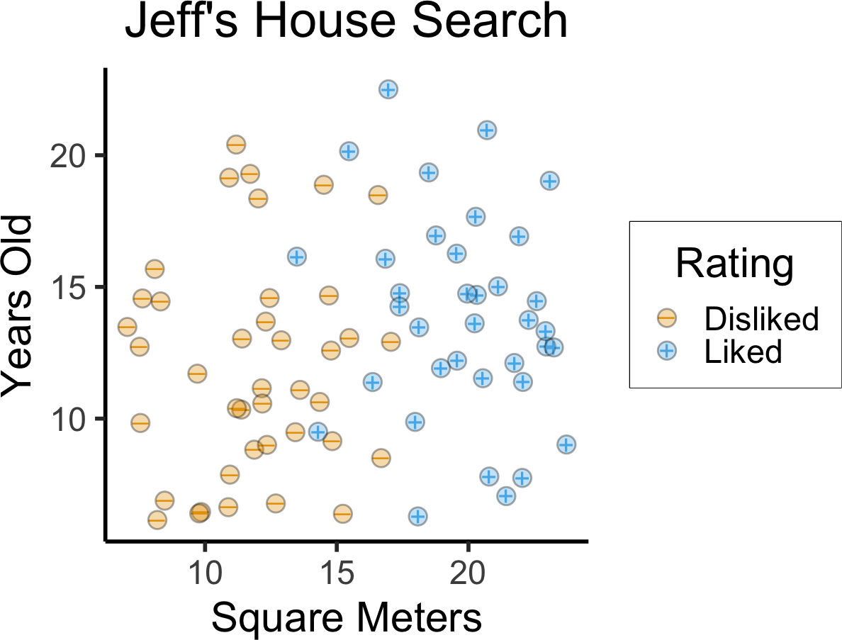
- Here we need to keep in mind how our goal is relative to the Data-Generating Process!
No Separating Hyperplane? 😧

- Don’t let the perfect be the enemy of the good!
Perfect vs. Good
- In fact, “sub-optimal” may be better than optimal, in terms of overfitting!

ISLR Figure 9.5: Notice how the dashed line on the right side may be better in terms of generalization, even though the solid line is the optimal Max-Margin Hyperplane!
“Slack” Variables
- The \(\varepsilon_i\) values also give us valuable information!
- \(\varepsilon_i = 0 \implies\) observation \(i\) on correct side of margin
- \(0 < \varepsilon_i \leq 1 \implies\) observation \(i\) is within margin but on correct side of hyperplane
- \(\varepsilon_i > 1 \implies\) observation \(i\) on wrong side of hyperplane

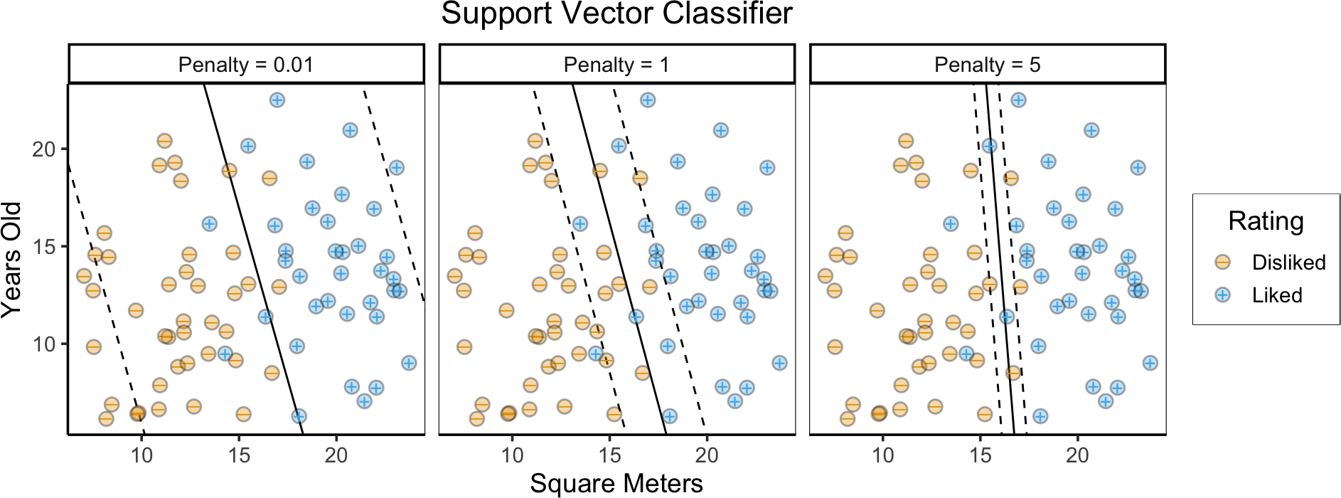
Our Non-Linearly-Separable Example
Code
library(e1071)
liked <- as.factor(nonsep_df$Rating == "Liked")
nonsep_cent_df <- nonsep_df
nonsep_cent_df$sqm <- scale(nonsep_cent_df$sqm)
nonsep_cent_df$yrs <- scale(nonsep_cent_df$yrs)
# Compute boundary for different cost budgets
budget_vals <- c(0.01, 1, 5)
svm_df <- tibble(
  sep_slope=numeric(), sep_intercept=numeric(),
  inv_slope=numeric(), inv_intercept=numeric(),
  margin_intercept=numeric(), margin_intercept_inv=numeric(),
  budget=numeric(), budget_label=character()
)
for (cur_c in budget_vals) {
  # print(cur_c)
  svm_model <- svm(liked ~ sqm + yrs, data=nonsep_cent_df, kernel="linear", cost=cur_c)
  cf <- coef(svm_model)
  sep_intercept <- -cf[1] / cf[3]
  sep_slope <- -cf[2] / cf[3]
  # Invert Z-scores
  sd_ratio <- sd(nonsep_df$yrs) / sd(nonsep_df$sqm)
  inv_slope <- sd_ratio * sep_slope
  inv_intercept <- mean(nonsep_df$yrs) - inv_slope * mean(nonsep_df$sqm) + sd(nonsep_df$yrs)*sep_intercept
  # And the margin boundary
  sv_index <- svm_model$index[1]
  sv_sqm <- nonsep_df$sqm[sv_index]
  sv_yrs <- nonsep_df$yrs[sv_index]
  margin_intercept <- sv_yrs - inv_slope * sv_sqm
  margin_diff <- inv_intercept - margin_intercept
  margin_intercept_inv <- inv_intercept + margin_diff
  cur_svm_row <- tibble_row(
    budget = cur_c,
    budget_label = paste0("Penalty = ",cur_c),
    sep_slope = sep_slope,
    sep_intercept = sep_intercept,
    inv_slope = inv_slope,
    inv_intercept = inv_intercept,
    margin_intercept = margin_intercept,
    margin_intercept_inv = margin_intercept_inv
  )
  svm_df <- bind_rows(svm_df, cur_svm_row)
}
ggplot() +
  # xlim(6,25) + ylim(2,22) +
  coord_equal() +
  # 45 is minus sign, 95 is em-dash
  scale_shape_manual(values=c(95, 43)) +
  theme_dsan(base_size=14) +
  geom_abline(
    data=svm_df,
    aes(intercept=inv_intercept, slope=inv_slope),
    linetype="solid"
  ) +
  geom_abline(
    data=svm_df,
    aes(intercept=margin_intercept, slope=inv_slope),
    linetype="dashed"
  ) +
  geom_abline(
    data=svm_df,
    aes(intercept=margin_intercept_inv, slope=inv_slope),
    linetype="dashed"
  ) +
  geom_point(
    data=nonsep_df,
    aes(x=sqm, y=yrs, color=Rating, shape=Rating), size=g_pointsize * 0.1,
    stroke=5
  ) +
  geom_point(
    data=nonsep_df,
    aes(x=sqm, y=yrs, fill=Rating), color='black', shape=21, size=3, stroke=0.75, alpha=0.333
  ) +
  labs(
    title = "Support Vector Classifier",
    x = "Square Meters",
    y = "Years Old"
  ) +
  facet_wrap(vars(budget_label), nrow=1) +
  theme(
    panel.border = element_rect(color = "black", fill = NA, size = 0.4)
  )
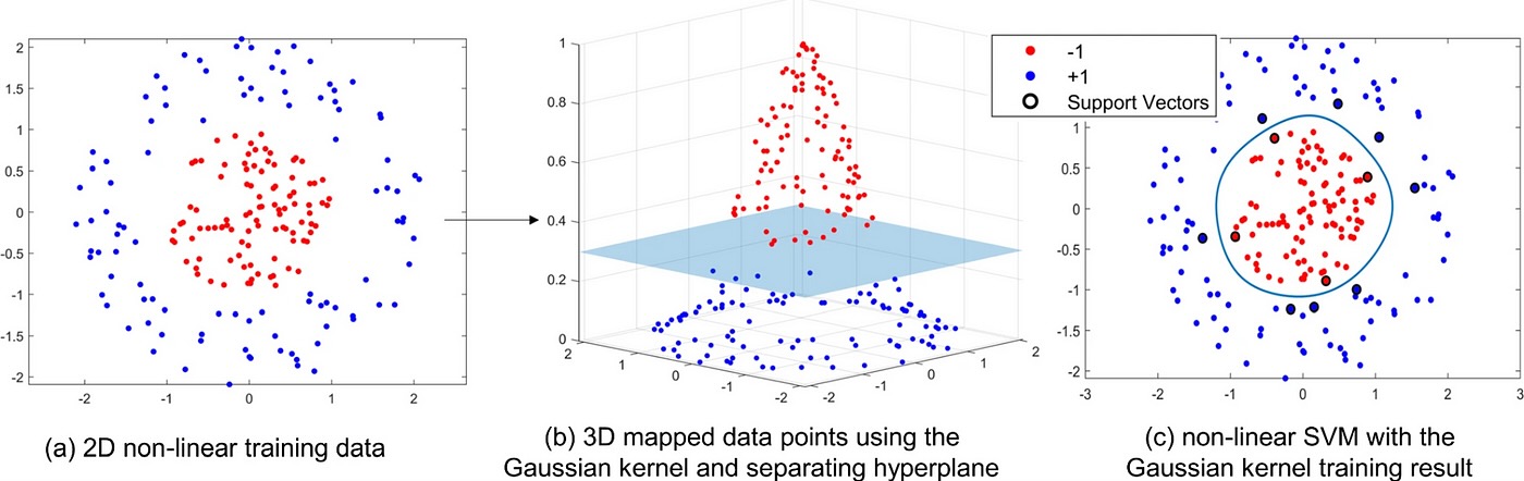
But… Why Restrict Ourselves to Lines?
- We just spent 7 weeks learning how to move from linear to non-linear! Basic template:
\[ \text{Nonlinear model} = \text{Linear model} \underbrace{- \; \text{linearity restriction}}_{\text{Enables overfitting...}} \underbrace{+ \text{ Complexity penalty}}_{\text{Prevent overfitting}} \]
- So… We should be able to find reasonable non-linear boundaries!

From MathWorks
Linear \(\rightarrow\) Linear
- Old feature space: \(\mathcal{S} = \{X_1, \ldots, X_J\}\)
- New feature space: \(\mathcal{S}^2 = \{X_1, X_1^2, \ldots, X_J, X_J^2\}\)
- Linear boundary in \(\mathcal{S}^2\) \(\implies\) Quadratic boundary in \(\mathcal{S}\)
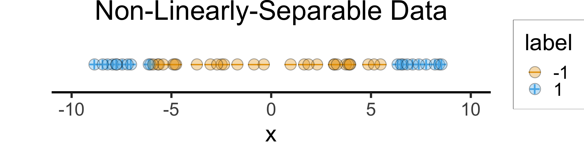
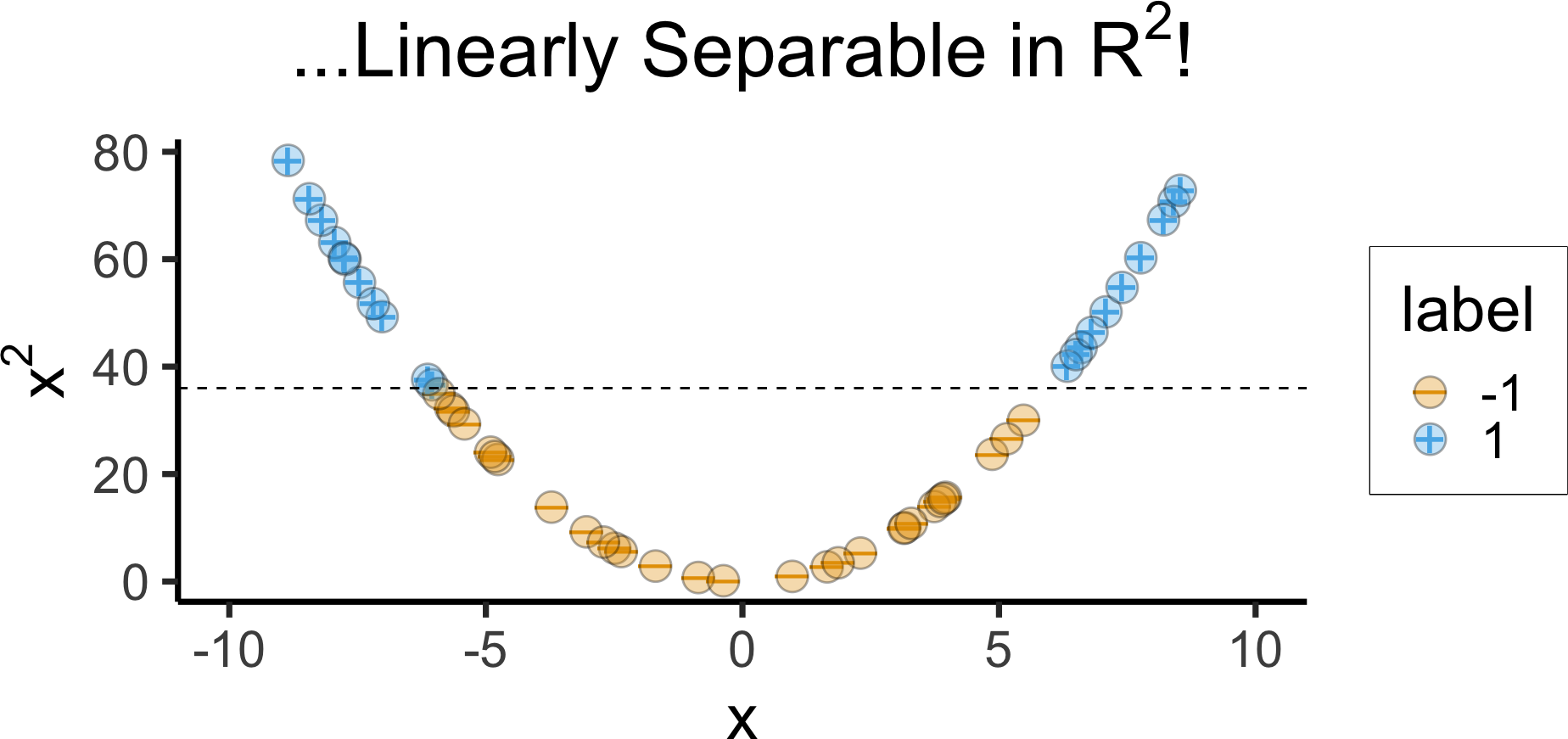
- Helpful example: Non-linearly separable in 1D \(\leadsto\) Linearly separable in 2D
1D Hyperplane = point! But no separating point here 😰
Code
library(latex2exp) |> suppressPackageStartupMessages()
x_vals <- runif(50, min=-9, max=9)
data_df <- tibble(x=x_vals) |> mutate(
  label = factor(ifelse(abs(x) >= 6, 1, -1)),
  x2 = x^2
)
data_df |> ggplot(aes(x=x, y=0, color=label)) +
  geom_point(
    aes(color=label, shape=label), size=g_pointsize,
    stroke=6
  ) +
  geom_point(
    aes(fill=label), color='black', shape=21, size=6, stroke=0.75, alpha=0.333
  ) +
  # xlim(6,25) + ylim(2,22) +
  # coord_equal() +
  # 45 is minus sign, 95 is em-dash
  scale_shape_manual(values=c(95, 43)) +
  theme_dsan(base_size=28) +
  theme(
    axis.line.y = element_blank(),
    axis.text.y = element_blank(),
    axis.ticks.y = element_blank(),
    axis.title.y = element_blank()
  ) +
  xlim(-10, 10) +
  ylim(-0.1, 0.1) +
  labs(title="Non-Linearly-Separable Data") +
  theme(
    plot.margin = unit(c(0,0,0,20), "mm")
  )
Code
data_df |> ggplot(aes(x=x, y=x2, color=label)) +
  geom_point(
    aes(color=label, shape=label), size=g_pointsize,
    stroke=6
  ) +
  geom_point(
    aes(fill=label), color='black', shape=21, size=6, stroke=0.75, alpha=0.333
  ) +
  geom_hline(yintercept=36, linetype="dashed") +
  # xlim(6,25) + ylim(2,22) +
  # coord_equal() +
  # 45 is minus sign, 95 is em-dash
  scale_shape_manual(values=c(95, 43)) +
  theme_dsan(base_size=28) +
  xlim(-10, 10) +
  labs(
    title = TeX("...Linearly Separable in $R^2$!"),
    y = TeX("$x^2$")
  )
And in 3D…
The Magic of Kernels
Radial Basis Function (RBF) Kernel:
\[ K(x_i, x_{i'}) = \exp\left[ -\gamma \sum_{j=1}^{J} (x_{ij} - x_{i'j})^2 \right] \]
Code
library(kernlab) |> suppressPackageStartupMessages()
library(mlbench) |> suppressPackageStartupMessages()
if (!file.exists("assets/linspike_df.rds")) {
  set.seed(5300)
  N <- 120
  x1_vals <- runif(N, min=-5, max=5)
  x2_raw <- x1_vals
  x2_noise <- rnorm(N, mean=0, sd=1.25)
  x2_vals <- x2_raw + x2_noise
  linspike_df <- tibble(x1=x1_vals, x2=x2_vals) |>
    mutate(
      label = factor(ifelse(x1^2 + x2^2 <= 2.75, 1, -1))
    )
  linspike_svm <- ksvm(
    label ~ x1 + x2,
    data = linspike_df,
    kernel = "rbfdot",
    C = 500,
    prob.model = TRUE
  )
  # Grid over which to evaluate decision boundaries
  npts <- 500
  lsgrid <- expand.grid(
    x1 = seq(from = -5, 5, length = npts),
    x2 = seq(from = -5, 5, length = npts)
  )
  # Predicted probabilities (as a two-column matrix)
  prob_svm <- predict(
    linspike_svm,
    newdata = lsgrid,
    type = "probabilities"
  )
  # Add predicted class probabilities
  lsgrid2 <- lsgrid |>
    cbind("SVM" = prob_svm[, 1L]) |>
    tidyr::gather(Model, Prob, -x1, -x2)

  # Serialize for quicker rendering
  saveRDS(linspike_df, "assets/linspike_df.rds")
  saveRDS(lsgrid2, "assets/lsgrid2.rds")
} else {
  linspike_df <- readRDS("assets/linspike_df.rds")
  lsgrid2 <- readRDS("assets/lsgrid2.rds")
}
linspike_df <- linspike_df |> mutate(
  Label = label
)
linspike_df |> ggplot(aes(x = x1, y = x2)) +
  # geom_point(aes(shape = label, color = label), size = 3, alpha = 0.75) +
  geom_point(aes(shape = Label, color = Label), size = 3, stroke=4) +
  geom_point(aes(fill=Label), color='black', shape=21, size=4, stroke=0.75, alpha=0.4) +
  xlab(expression(X[1])) +
  ylab(expression(X[2])) +
  coord_fixed() +
  theme(legend.position = "none") +
  theme_dsan(base_size=28) +
  xlim(-5, 5) + ylim(-5, 5) +
  stat_contour(
    data = lsgrid2,
    aes(x = x1, y = x2, z = Prob),
    breaks = 0.5,
    color = "black"
  ) +
  scale_shape_manual(values=c(95, 43))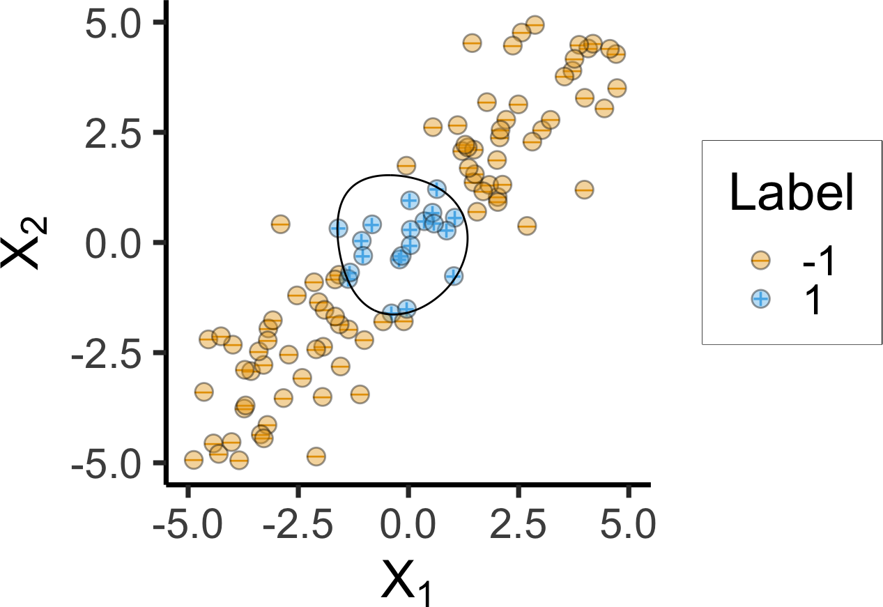
Code
if (!file.exists("assets/spiral_df.rds")) {
  spiral_df <- as.data.frame(
    mlbench.spirals(300, cycles = 2, sd = 0.09)
  )
  names(spiral_df) <- c("x1", "x2", "label")

  # Fit SVM using a RBF kernel
  spirals_svm <- ksvm(
    label ~ x1 + x2,
    data = spiral_df,
    kernel = "rbfdot",
    C = 500,
    prob.model = TRUE
  )

  # Grid over which to evaluate decision boundaries
  npts <- 500
  xgrid <- expand.grid(
    x1 = seq(from = -2, 2, length = npts),
    x2 = seq(from = -2, 2, length = npts)
  )

  # Predicted probabilities (as a two-column matrix)
  prob_svm <- predict(
    spirals_svm,
    newdata = xgrid,
    type = "probabilities"
  )

  # Add predicted class probabilities
  xgrid2 <- xgrid |>
    cbind("SVM" = prob_svm[, 1L]) |>
    tidyr::gather(Model, Prob, -x1, -x2)

  # Serialize for quicker rendering
  saveRDS(spiral_df, "assets/spiral_df.rds")
  saveRDS(xgrid2, "assets/xgrid2.rds")
} else {
  spiral_df <- readRDS("assets/spiral_df.rds")
  xgrid2 <- readRDS("assets/xgrid2.rds")
}
# And plot
spiral_df <- spiral_df |> mutate(
  Label = factor(ifelse(label == 2, 1, -1))
)
spiral_df |> ggplot(aes(x = x1, y = x2)) +
  geom_point(aes(shape = Label, color = Label), size = 3, stroke=4) +
  geom_point(aes(fill=Label), color='black', shape=21, size=4, stroke=0.75, alpha=0.4) +
  xlab(expression(X[1])) +
  ylab(expression(X[2])) +
  xlim(-2, 2) +
  ylim(-2, 2) +
  coord_fixed() +
  theme(legend.position = "none") +
  theme_dsan(base_size=28) +
  stat_contour(
    data = xgrid2,
    aes(x = x1, y = x2, z = Prob),
    breaks = 0.5,
    color = "black"
  ) +
  scale_shape_manual("Label", values=c(95, 43))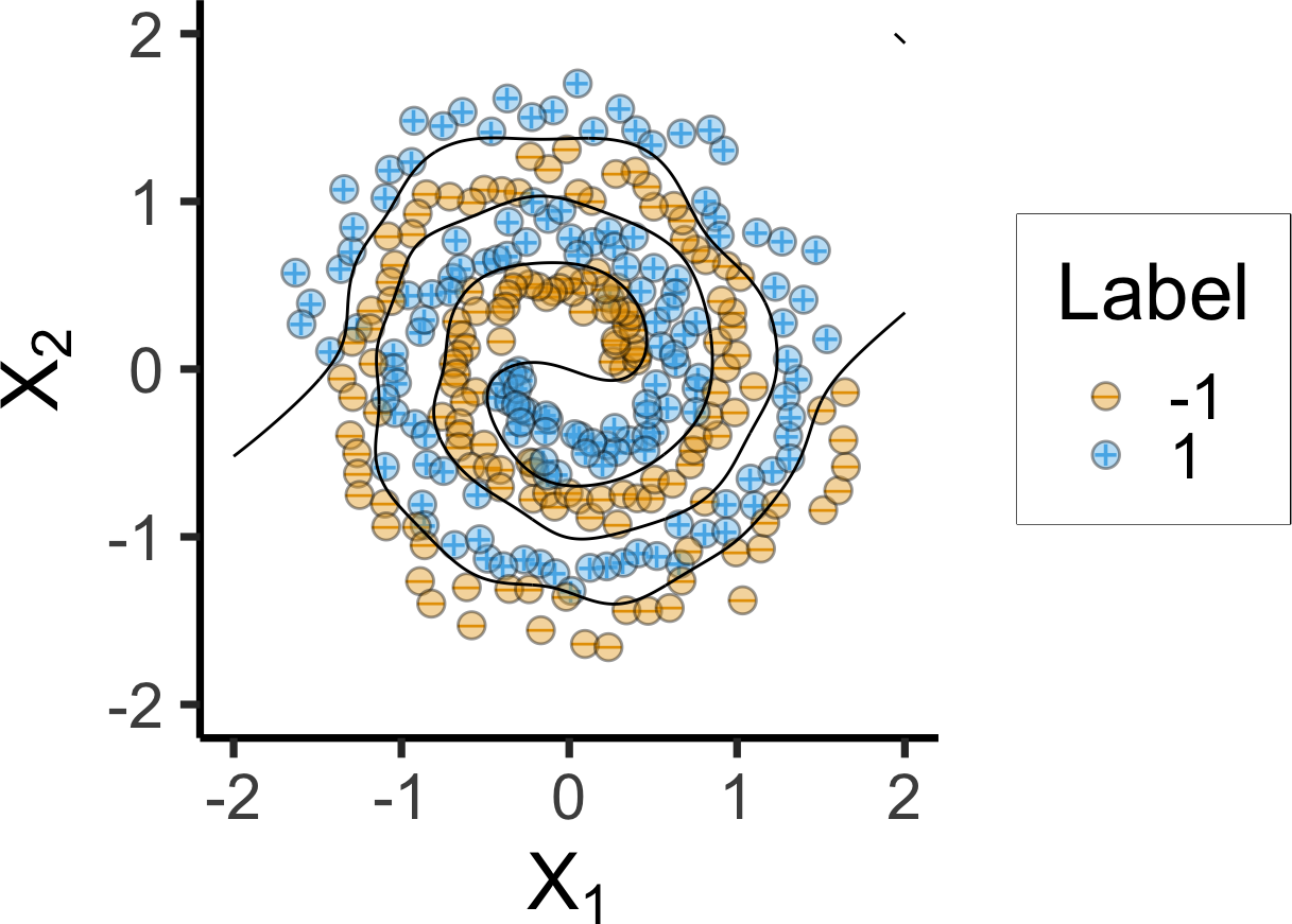
Inner Products are Already Similarities!
- When linearly separable, this is exactly the property we use (by computing inner product of new vector \(\mathbf{x}\) with support vectors \(\mathbf{x}_i\)) to classify!

- Why restrict ourselves to this similarity function? Choosing \(K\) converts the problem:
- From finding transformation of features allowing linear separability
- To finding similarity function for observations allowing linear separability