Week 7: Basis Functions and Splines
DSAN 5300: Statistical Learning
Spring 2025, Georgetown University
Monday, February 24, 2025
What’s So Bad About Polynomial Regression?
- Mathematically, Weierstrass Approximation Theorem says we can model any function as (possibly infinite) sum of polynomials
- In practice, this can be a horrifically bad way to actually model things:
Raw data: \(y = \sin(x) + \varepsilon\)
Code
library(tidyverse) |> suppressPackageStartupMessages()
library(latex2exp) |> suppressPackageStartupMessages()
N <- 200
x_vals <- seq(from=-10, to=10, length.out=N)
y_raw <- sin(x_vals)
y_noise <- rnorm(length(y_raw), mean=0, sd=0.075)
y_vals <- y_raw + y_noise
dgp_label <- TeX("Raw Data")
data_df <- tibble(x=x_vals, y=y_vals)
base_plot <- data_df |> ggplot(aes(x=x, y=y)) +
  geom_point() +
  theme_dsan(base_size=28)
base_plot + labs(title=dgp_label)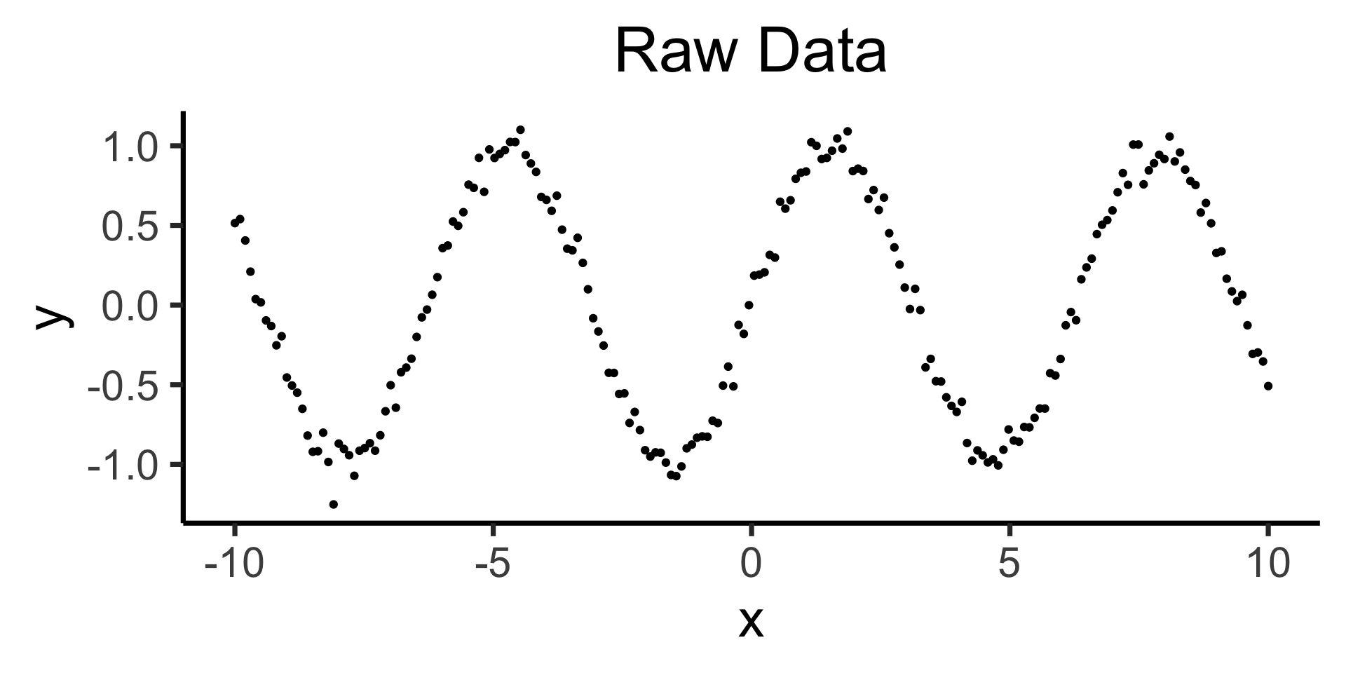
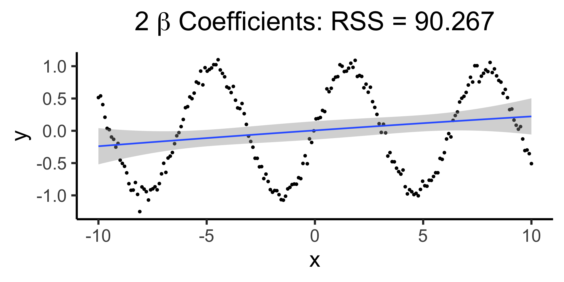
Bad (quadratic) model
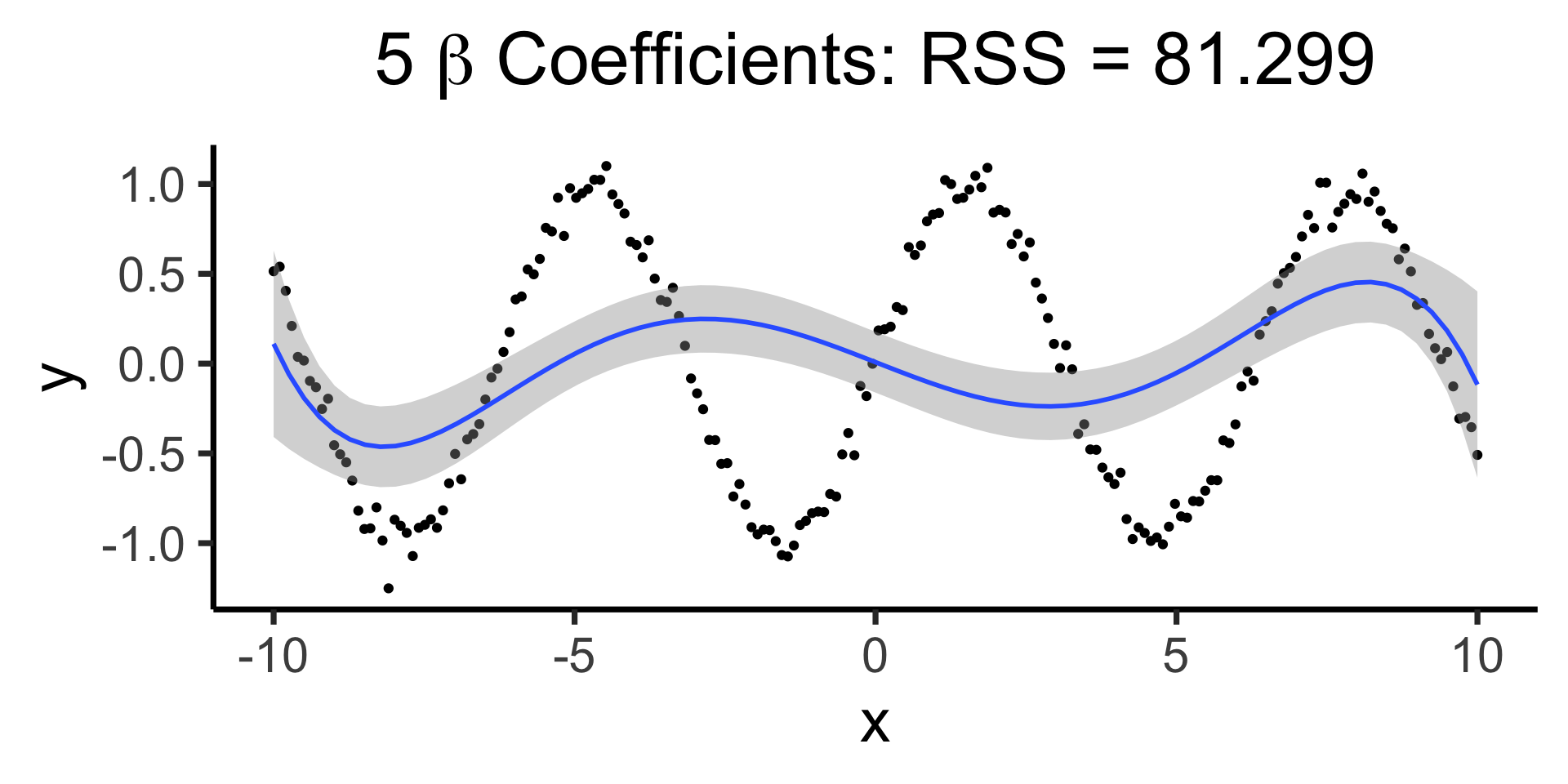
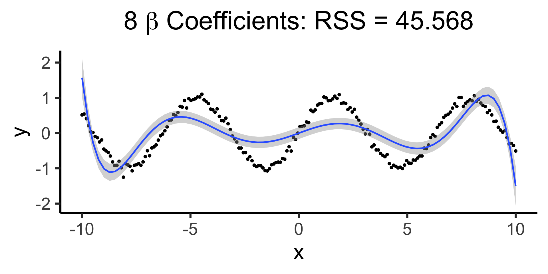
Making it “better” with more complex polynomials
Code
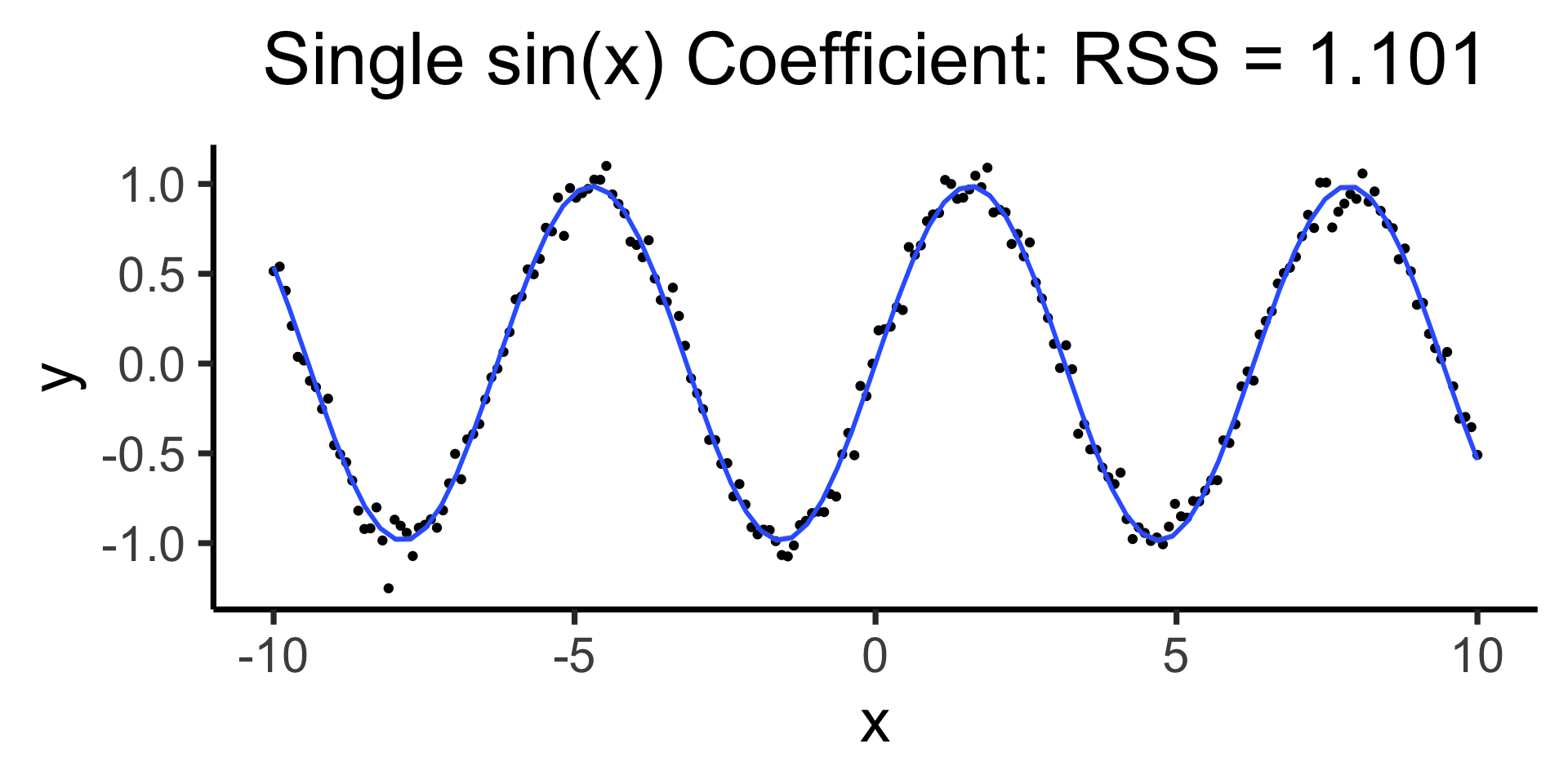
Using all data to estimate single parameter, by using the “correct” basis function!
\[ Y = \beta_0 + \beta_1 \sin(x) \]
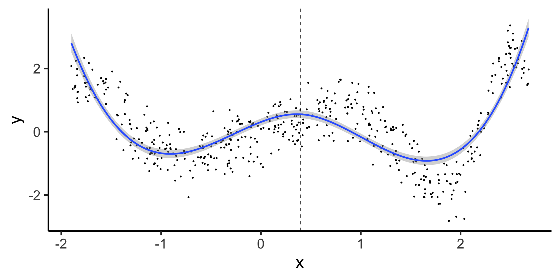
Discontinuous Segmented Regression
- Here we see why our first two basis functions were polynomial and piecewise: most rudimentary spline fits a polynomial to each piece
Code
library(tidyverse) |> suppressPackageStartupMessages()
set.seed(5300)
compute_y <- function(x) {
  return(x * cos(x^2))
}
N <- 500
xmin <- -1.9
xmax <- 2.7
x_vals <- runif(N, min=xmin, max=xmax)
y_raw = compute_y(x_vals)
y_noise = rnorm(N, mean=0, sd=0.5)
y_vals <- y_raw + y_noise
prod_df <- tibble(x=x_vals, y=y_vals)
knot <- (xmin + xmax) / 2
prod_df <- prod_df |> mutate(segment = x <= knot)
# First segment model
#left_df <- prod_df |> filter(x <= knot_point)
#left_model <- lm(y ~ poly(x, 2), data=left_df)
prod_df |> ggplot(aes(x=x, y=y, group=segment)) +
  geom_point(size=0.5) +
  geom_vline(xintercept=knot, linetype="dashed") +
  geom_smooth(method='lm', formula=y ~ poly(x, 2), se=TRUE) +
  theme_classic(base_size=22)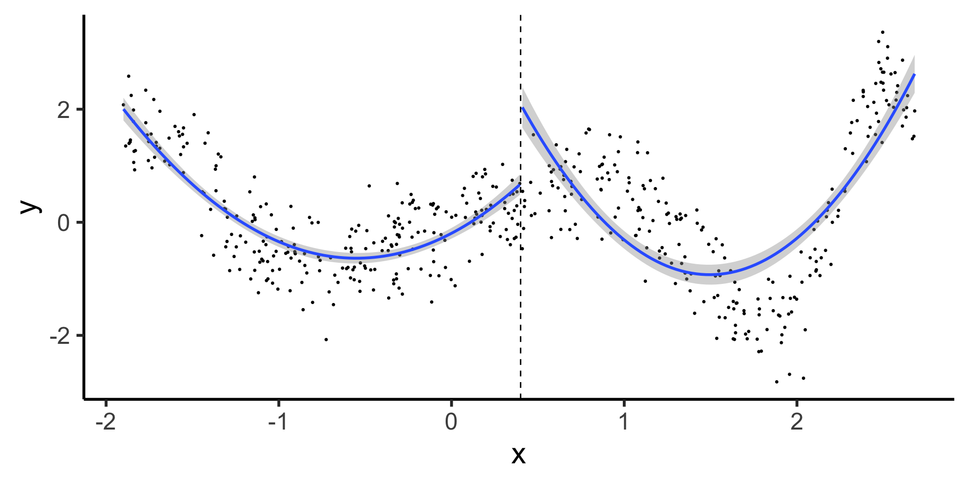
- What’s the issue with this?
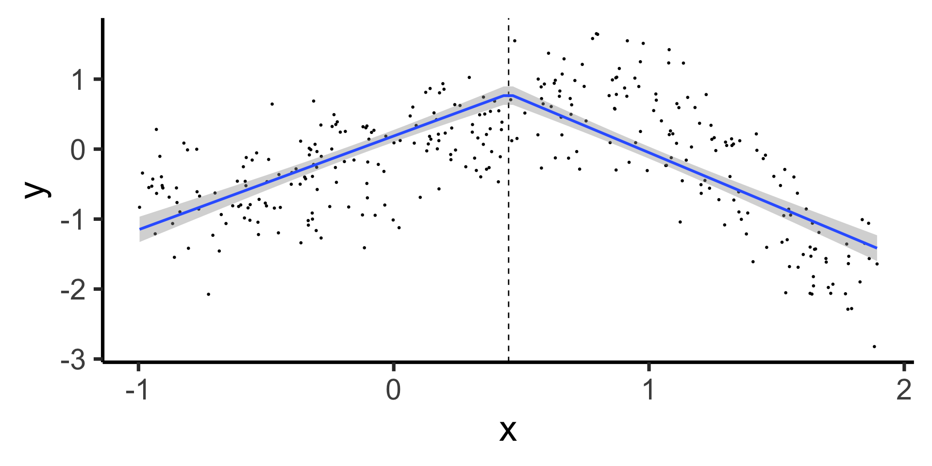
Forcing Continuity at Knot Points
- Starting slow: let’s come back down to line world…
- Why are these two lines “allowed” to be non-continuous, under our current approach?
\[ \hspace{6.5cm} Y^{\phantom{🧐}}_L = \beta_0 + \beta_1 X_L \]
\[ Y_R = \beta_0^{🧐} + \beta_1 X_R \hspace{5cm} \]
Code
set.seed(5300)
xmin_sub <- -1
xmax_sub <- 1.9
sub_df <- prod_df |> filter(x >= xmin_sub & x <= xmax_sub)
sub_knot <- (xmin_sub + xmax_sub) / 2
sub_df <- sub_df |> mutate(segment = x <= sub_knot)
# First segment model
sub_df |> ggplot(aes(x=x, y=y, group=segment)) +
  geom_point(size=0.5) +
  geom_vline(xintercept=sub_knot, linetype="dashed") +
  geom_smooth(method='lm', formula=y ~ x, se=TRUE, linewidth=g_linewidth) +
  theme_classic(base_size=28)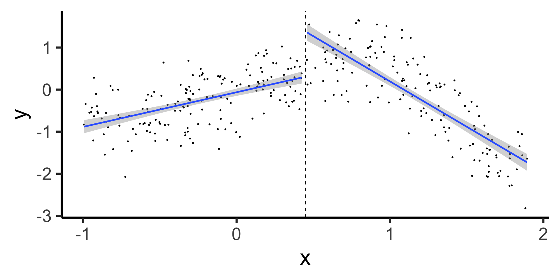
- …We need \(X_R\) to have its own slope but not its own intercept! Something like:
\[ Y = \beta_0 + \beta_1 (X \text{ before } \xi) + \beta_2 (X \text{ after } \xi) \]
Truncated Power Basis (ReLU Basis)
\[ \text{ReLU}(x) \definedas (x)_+ \definedas \begin{cases} 0 &\text{if }x \leq 0 \\ x &\text{if }x > 0 \end{cases} \implies (x - \xi)_+ = \begin{cases} 0 &\text{if }x \leq \xi \\ x - \xi &\text{if }x > 0 \end{cases} \]
Code
library(latex2exp) |> suppressPackageStartupMessages()
trunc_x <- function(x, xi) {
  return(ifelse(x <= xi, 0, x - xi))
}
trunc_x_05 <- function(x) trunc_x(x, 1/2)
trunc_title <- TeX("$(x - \\xi)_+$ with $\\xi = 0.5$")
trunc_label <- TeX("$y = (x - \\xi)_+$")
ggplot() +
  stat_function(
    data=data.frame(x=c(-3,3)),
    fun=trunc_x_05,
    linewidth=g_linewidth
  ) +
  xlim(-3, 3) +
  theme_dsan(base_size=28) +
  labs(
    title = trunc_title,
    x = "x",
    y = trunc_label
  )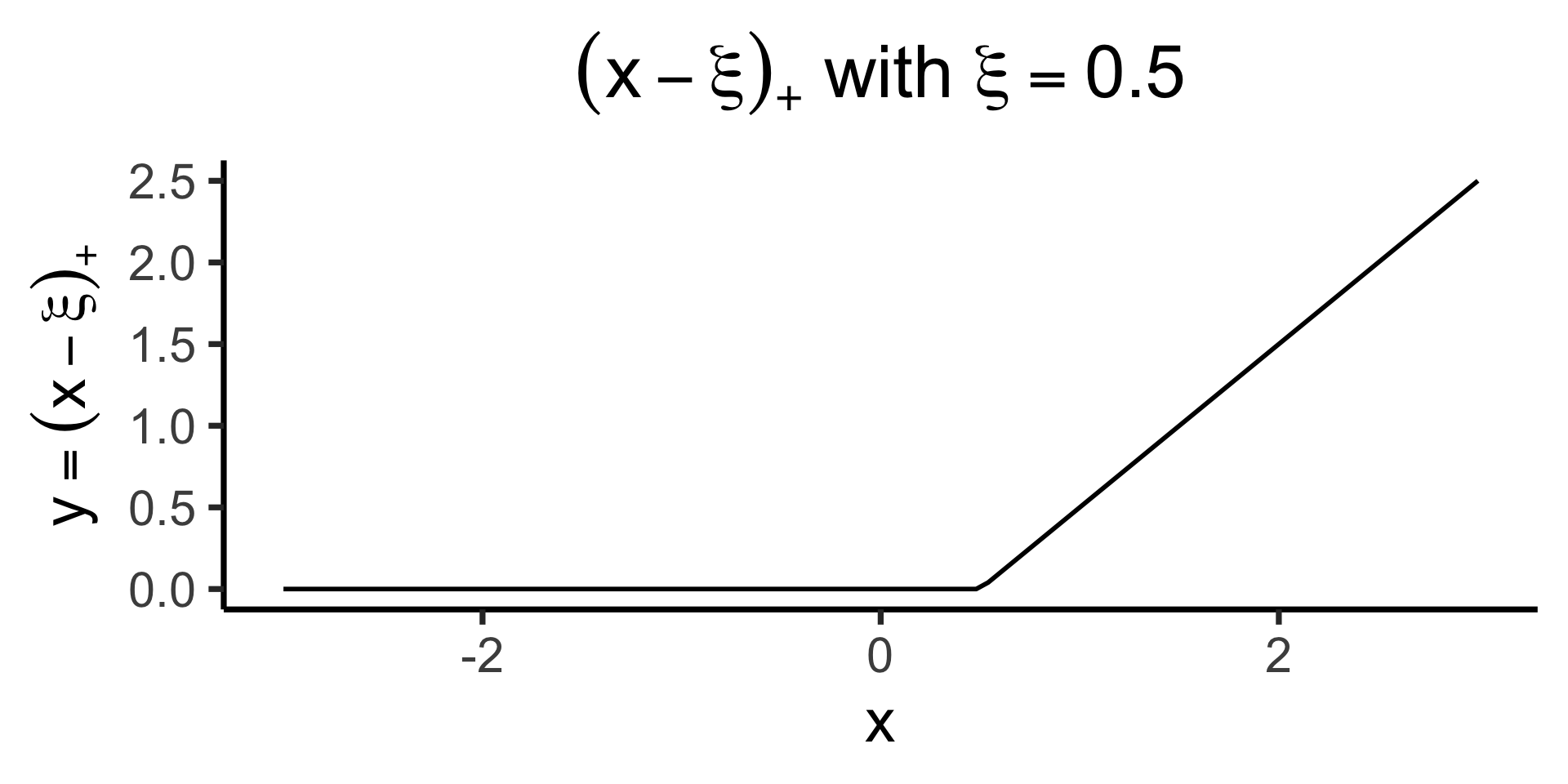
- \(\Rightarrow\) we can include a “slope modifier” \(\beta_m (X - \xi)_+\) that only “kicks in” once \(x\) goes past \(\xi\)! (Changing slope by \(\beta_m\))
Linear Segments with Continuity at Knot
Our new (non-naïve) model:
\[ \begin{align*} Y &= \beta_0 + \beta_1 X + \beta_2 (X - \xi)_+ \\ &= \beta_0 + \begin{cases} \beta_1 X &\text{if }X \leq \xi \\ (\beta_1 + \beta_2)X &\text{if }X > \xi \end{cases} \end{align*} \]
Code
| term | estimate | std.error | statistic |
|---|---|---|---|
| (Intercept) | 0.187 | 0.044 | 4.255 |
| x | 1.340 | 0.093 | 14.342 |
| x_tr | -2.868 | 0.168 | -17.095 |
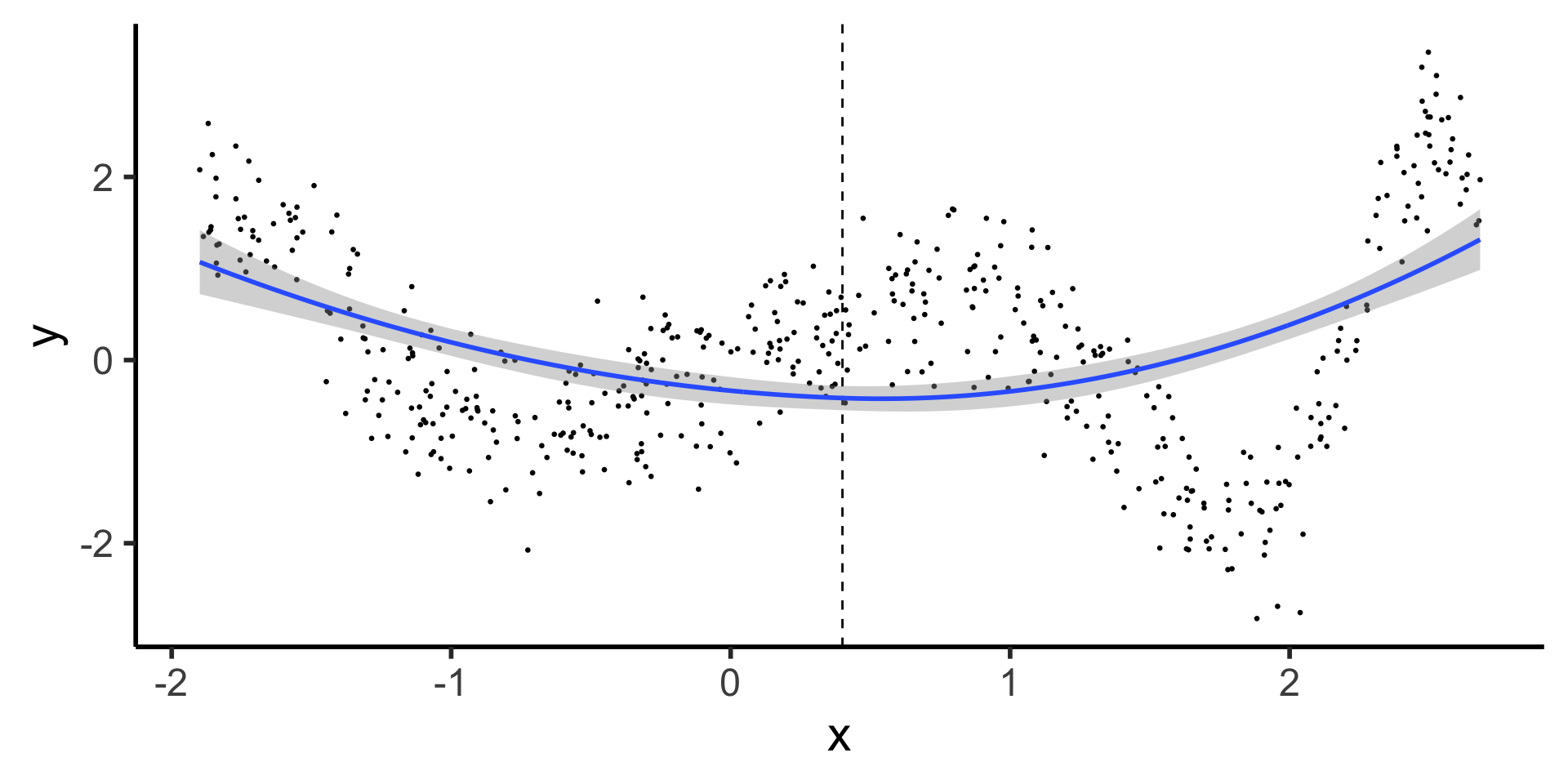
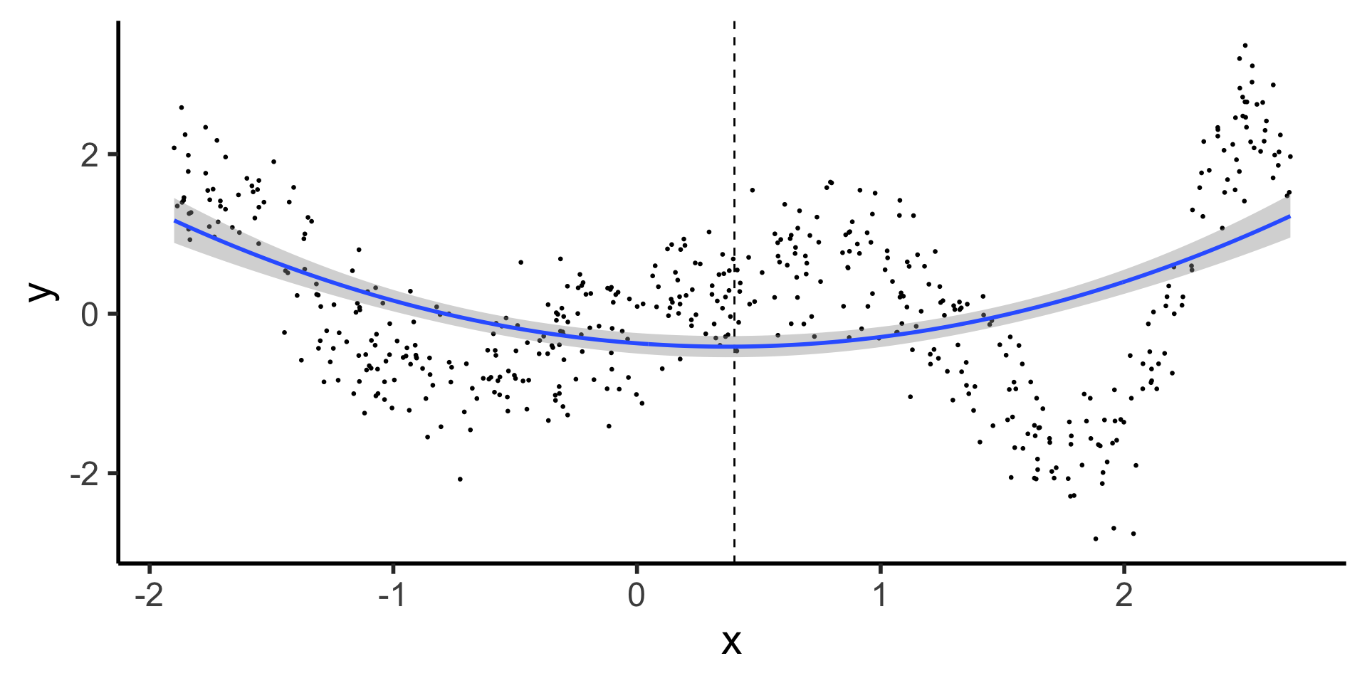
Continuous Segmented Regression
\[ \begin{align*} Y &= \beta_0 + \beta_1 X + \beta_2 X^2 + \beta_3 (X - \xi)_+ + \beta_4 (X - \xi)_+^2 \\[0.8em] &= \beta_0 + \begin{cases} \beta_1 X + \beta_2 X^2 &\text{if }X \leq \xi \\ (\beta_1 + \beta_3) X + (\beta_2 + \beta_4) X^2 &\text{if }X > \xi \end{cases} \end{align*} \]
Code
cont_seg_plot <- ggplot() +
  geom_point(data=prod_df, aes(x=x, y=y), size=0.5) +
  geom_vline(xintercept=knot, linetype="dashed") +
  stat_smooth(
    data=prod_df, aes(x=x, y=y),
    method='lm',
    formula=y ~ poly(x,2) + poly(ifelse(x > knot, (x - knot), 0), 2),
    n = 300
  ) +
  #geom_smooth(data=prod_df |> filter(segment == FALSE), aes(x=x, y=y), method='lm', formula=y ~ poly(x,2)) +
  # geom_smooth(method=segreg, formula=y ~ seg(x, npsi=1, fixed.psi=0.5)) + # + seg(I(x^2), npsi=1)) +
  theme_classic(base_size=22)
cont_seg_plot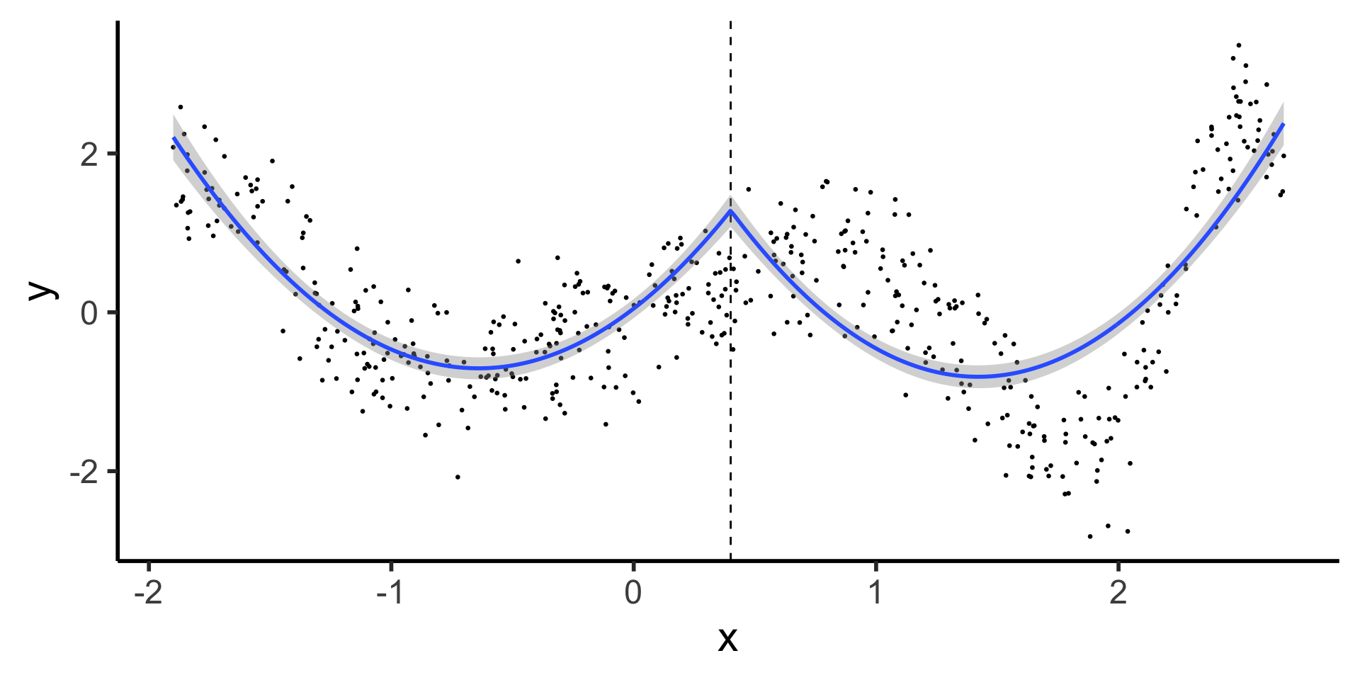
- There’s still a problem here… can you see what it is? (Hint: things that break calculus)
Constrained Derivatives: “Quadratic Splines” (⚠️)
- Like “Linear Probability Models”, “Quadratic Splines” are a red flag
- Why? If we have leftmost plot below, but want it differentiable everywhere… only option is to fit a single quadratic, defeating the whole point of the “chopping”!
\[ \frac{\partial Y}{\partial X} = \beta_1 + 2\beta_2 X + \beta_3 + 2\beta_4 X \]

“Quadratic Spline”:
- \(\implies\) Least-complex function that allows smooth “joining” is cubic function
Cubic Splines (aka, Splines)
(We did it, we finally did it)
Natural Splines: Why Not Stop There?
Polynomials start to BEHAVE BADLY as they go to \(-\infty\) and \(\infty\)
Code
library(splines) |> suppressPackageStartupMessages()
set.seed(5300)
N_sparse <- 400
x_vals <- runif(N_sparse, min=xmin, max=xmax)
y_raw = compute_y(x_vals)
y_noise = rnorm(N_sparse, mean=0, sd=1.0)
y_vals <- y_raw + y_noise
sparse_df <- tibble(x=x_vals, y=y_vals)
knot_sparse <- (xmin + xmax) / 2
knot_vec <- c(-1.8,-1.7,-1.6,-1.5,-1.4,-1.2,-1.0,-0.8,-0.6,-0.4,-0.2,0,knot_sparse,1,1.5,2)
knot_df <- tibble(knot=knot_vec)
# Boundary lines
left_bound_line <- geom_vline(
  xintercept = xmin + 0.1, linewidth=1,
  color="red", alpha=0.8
)
right_bound_line <- geom_vline(
  xintercept = xmax - 0.1,
  linewidth=1, color="red", alpha=0.8
)
ggplot() +
  geom_point(data=sparse_df, aes(x=x, y=y), size=0.5) +
  geom_vline(
    data=knot_df, aes(xintercept=knot),
    linetype="dashed"
  ) +
  stat_smooth(
    data=sparse_df, aes(x=x, y=y),
    method='lm',
    formula=y ~ bs(x, knots=c(knot_sparse), degree=25),
    n=300
  ) +
  left_bound_line +
  right_bound_line +
  theme_dsan(base_size=22)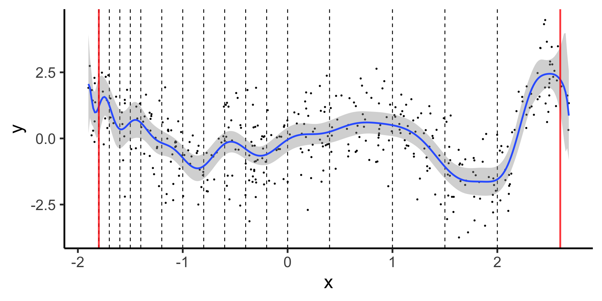
Natural Splines: Force leftmost and rightmost pieces to be linear
Code
library(splines) |> suppressPackageStartupMessages()
set.seed(5300)
N_sparse <- 400
x_vals <- runif(N_sparse, min=xmin, max=xmax)
y_raw = compute_y(x_vals)
y_noise = rnorm(N_sparse, mean=0, sd=1.0)
y_vals <- y_raw + y_noise
sparse_df <- tibble(x=x_vals, y=y_vals)
knot_sparse <- (xmin + xmax) / 2
ggplot() +
  geom_point(data=sparse_df, aes(x=x, y=y), size=0.5) +
  stat_smooth(
    data=sparse_df, aes(x=x, y=y),
    method='lm',
    formula=y ~ ns(x, knots=knot_vec, Boundary.knots=c(xmin + 0.1, xmax - 0.1)),
    n=300
  ) +
  geom_vline(
    data=knot_df, aes(xintercept=knot),
    linetype="dashed"
  ) +
  left_bound_line +
  right_bound_line +
  theme_dsan(base_size=22)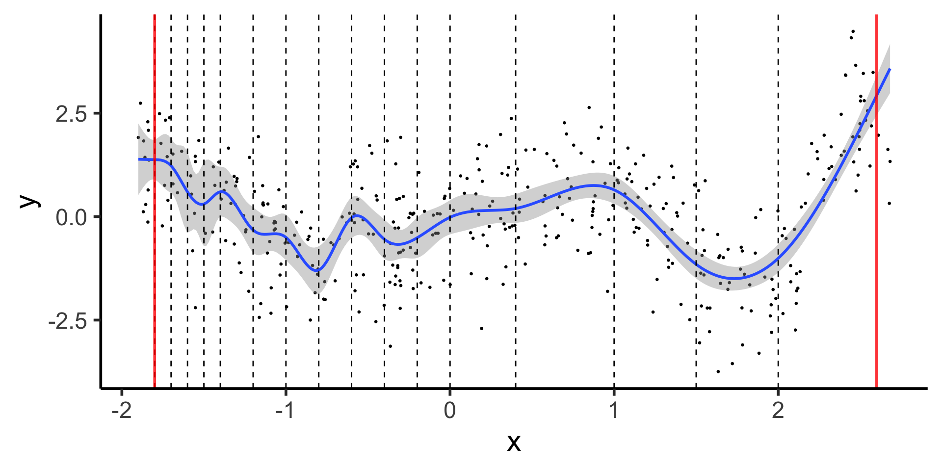
Reminder (W04): Penalizing Complexity
Week 4 (General Form):
\[ \boldsymbol\theta^* = \underset{\boldsymbol\theta}{\operatorname{argmin}} \left[ \mathcal{L}(y, \widehat{y}; \boldsymbol\theta) + \lambda \cdot \mathsf{Complexity}(\boldsymbol\theta) \right] \]

Last Week (Penalizing Polynomials):
\[ \boldsymbol\beta^*_{\text{lasso}} = \underset{\boldsymbol\beta, \lambda}{\operatorname{argmin}} \left[ \frac{1}{N}\sum_{i=1}^{N}(\widehat{y}_i(\boldsymbol\beta) - y_i)^2 + \lambda \|\boldsymbol\beta\|_1 \right] \]

Now (Penalizing Sharp Change / Wigglyness):
\[ g^* = \underset{g, \lambda}{\operatorname{argmin}} \left[ \sum_{i=1}^{N}(g(x_i) - y_i)^2 + \lambda \overbrace{\int}^{\mathclap{\text{Sum of}}} [\underbrace{g''(t)}_{\mathclap{\text{Change in }g'(t)}}]^2 \mathrm{d}t \right] \]