Week 4: The Scourge of Overfitting
DSAN 5300: Statistical Learning
Spring 2025, Georgetown University
Monday, February 3, 2025
What We Have Thus Far
- We have a core model, regression, that we can build up into p much anything we want!
| Class Topic | This Video |
|---|---|
| Linear regression | Pachelbel’s Canon in D (1m26s-1m46s) |
| Logistic regression | Add swing:  (1m46s) (1m46s) |
| Neural networks | (triads \(\mapsto\) 7th/9th chords) (5m24s-5m53s) |
…Can We Just, Like, Not?
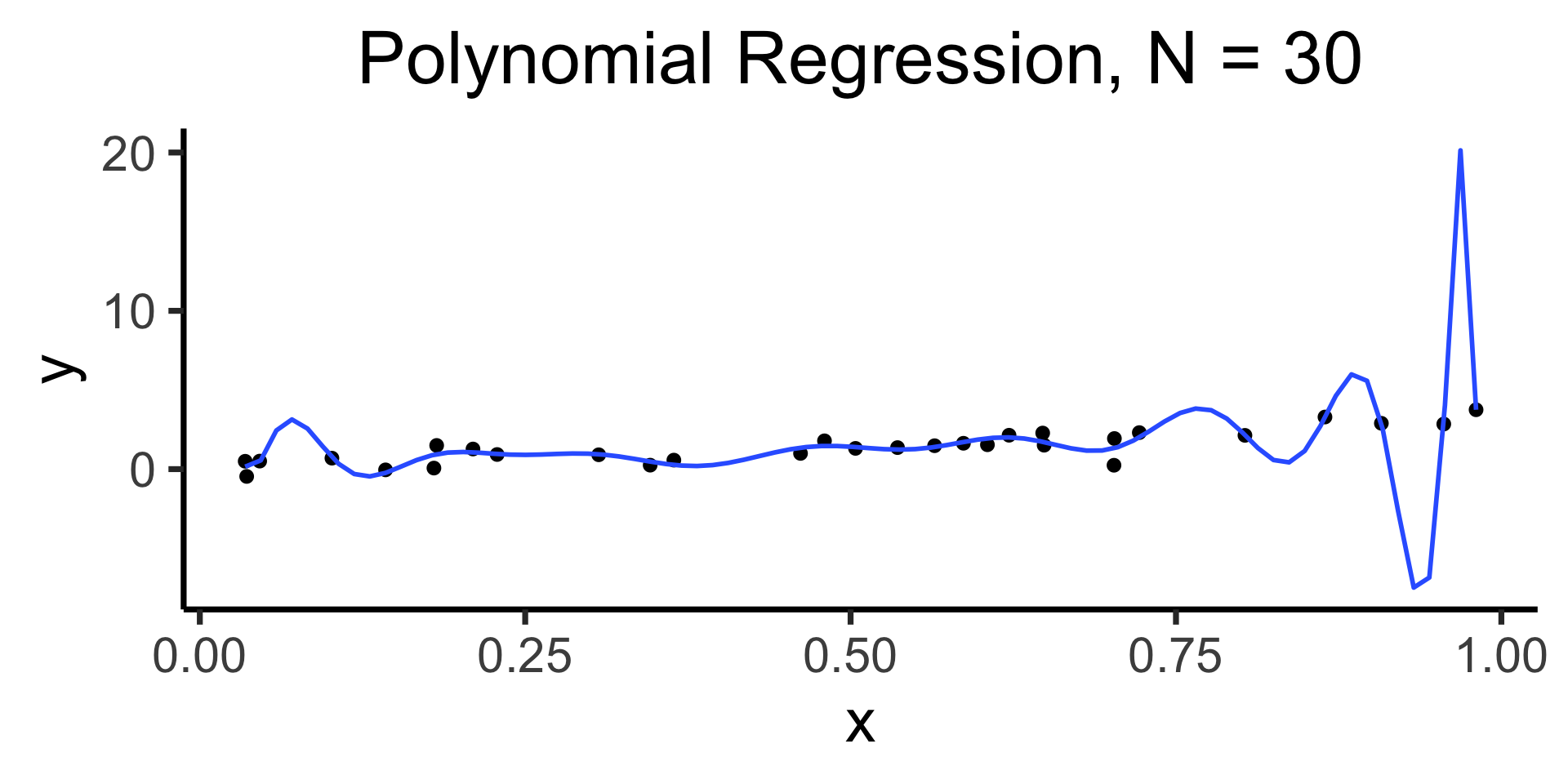
- What happens if we “unleash” fancier non-linear models on data the same way we’ve been using linear models?
- The evil scourge of… OVERFITTING (⚡️ a single overly-dramatic lightning bolt strikes the whiteboard behind me right at this exact moment what are the odds ⚡️)

Code
library(tidyverse)
set.seed(5300)
N <- 30
x_vals <- runif(N, min=0, max=1)
y_vals_raw <- 3 * x_vals
y_noise <- rnorm(N, mean=0, sd=0.5)
y_vals <- y_vals_raw + y_noise
data_df <- tibble(x=x_vals, y=y_vals)
data_df |> ggplot(aes(x=x, y=y)) +
  geom_point(size=2) +
  stat_smooth(
    method="lm",
    formula="y ~ x",
    se=FALSE,
    linewidth=1
  ) +
  labs(
    title = paste0("Linear Regression, N = ",N)
  ) +
  theme_dsan(base_size=28)
Memorizing Data vs. Learning the Relationship
Code
x <- seq(from = 0, to = 1, by = 0.1)
n <- length(x)
eps <- rnorm(n, 0, 0.04)
y <- x + eps
# But make one big outlier
midpoint <- ceiling((3/4)*n)
y[midpoint] <- 0
of_data <- tibble::tibble(x=x, y=y)
# Linear model
lin_model <- lm(y ~ x)
# But now polynomial regression
poly_model <- lm(y ~ poly(x, degree = 10, raw=TRUE))
#summary(model)
ggplot(of_data, aes(x=x, y=y)) +
  geom_point(size=g_pointsize/2) +
  labs(
    title = "Training Data",
    color = "Model"
  ) +
  theme_dsan(base_size=16)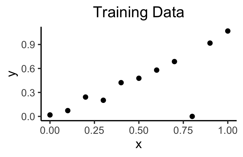
Code
ggplot(of_data, aes(x=x, y=y)) +
  geom_point(size=g_pointsize/2) +
  geom_abline(aes(intercept=0, slope=1, color="Linear"), linewidth=1, show.legend = FALSE) +
  stat_smooth(method = "lm",
              formula = y ~ poly(x, 10, raw=TRUE),
              se = FALSE, aes(color="Polynomial")) +
  labs(
    title = "A Perfect Model?",
    color = "Model"
  ) +
  theme_dsan(base_size=16)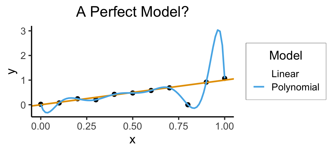
5000: Accuracy \(\leadsto\) 5300: Generalization
- Training Accuracy: How well does it fit the data we can see?
- Test Accuracy: How well does it generalize to future data?
Code
# Data setup
x_test <- seq(from = 0, to = 1, by = 0.1)
n_test <- length(x_test)
eps_test <- rnorm(n_test, 0, 0.04)
y_test <- x_test + eps_test
of_data_test <- tibble::tibble(x=x_test, y=y_test)
lin_y_pred_test <- predict(lin_model, as.data.frame(x_test))
#lin_y_pred_test
lin_resids_test <- y_test - lin_y_pred_test
#lin_resids_test
lin_rss_test <- sum(lin_resids_test^2)
#lin_rss_test
# Lin R2 = 1 - RSS/TSS
tss_test <- sum((y_test - mean(y_test))^2)
lin_r2_test <- 1 - (lin_rss_test / tss_test)
#lin_r2_test
# Now the poly model
poly_y_pred_test <- predict(poly_model, as.data.frame(x_test))
poly_resids_test <- y_test - poly_y_pred_test
poly_rss_test <- sum(poly_resids_test^2)
#poly_rss_test
# RSS
poly_r2_test <- 1 - (poly_rss_test / tss_test)
#poly_r2_test
ggplot(of_data, aes(x=x, y=y)) +
  stat_smooth(method = "lm",
              formula = y ~ poly(x, 10, raw = TRUE),
              se = FALSE, aes(color="Polynomial")) +
  theme_classic() +
  geom_point(data=of_data_test, aes(x=x_test, y=y_test), size=g_pointsize/2) +
  geom_abline(aes(intercept=0, slope=1, color="Linear"), linewidth=1, show.legend = FALSE) +
  labs(
    title = "Evaluation: Unseen Test Data",
    color = "Model"
  ) +
  theme_dsan(base_size=16)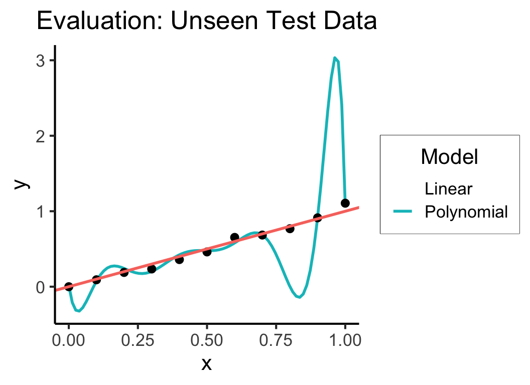
In Other Words…

Image source: circulated as secret shitposting among PhD students in seminars