Week 8: Statistical Inference
DSAN 5100: Probabilistic Modeling and Statistical Computing
Section 01
Tuesday, October 21, 2025
Finite-State Automata
(Deterministic!) Only “accepts” strings with even number of 1s:

| Input String | Result | Input String | Result |
|---|---|---|---|
| \(\varepsilon\) | ✅ | 01 |
|
0 |
✅ | 10 |
|
1 |
1000000 |
||
00 |
✅ | 10000001 |
✅ |
- …But we’re trying to model probabilistic evolution!
Enter Markov Chains


\[ \begin{array}{c c} & \begin{array}{c c c} 1\phantom{1} & \phantom{1}2\phantom{1} & \phantom{1}3 \\ \end{array} \\ \begin{array}{c c c}1 \\ 2 \\ 3 \end{array} & \left[ \begin{array}{c c c} 0 & 1/2 & 1/2 \\ 1/3 & 0 & 2/3 \\ 1/3 & 2/3 & 0 \end{array} \right] \end{array} \]
\[ \begin{array}{c c} & \begin{array}{c c c} 1\phantom{1} & \phantom{2}2\phantom{2} & \phantom{1}3 \\ \end{array} \\ \begin{array}{c c c}1 \\ 2 \\ 3 \end{array} & \left[ \begin{array}{c c c} 1/2 & 1/3 & 1/6 \\ 1/10 & 1/2 & 2/5 \\ 1/8 & 3/8 & 1/2 \end{array} \right] \end{array} \]

PageRank (Matrix Magic)
- What is the relevance of this abstract topic? …🤑
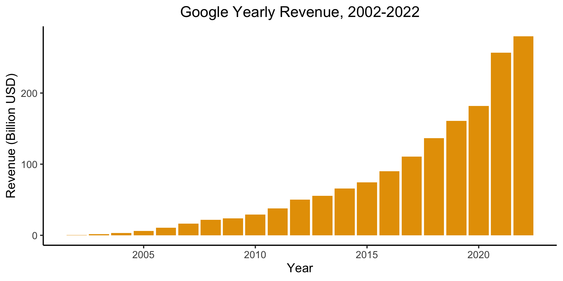
- PageRank = The “spark” that ignited the Google flame
PageRank Visualized
- Nodes = Webpages, Edges = Links

- Goal: Rank the relative “importance” of a site \(S_i\), taking into account the importance of other sites that link to \(S_i\)
- “Important” sites: linked to often, and linked to often by other important sites
Zooming in on Euclid


→
Inference

Stability out of Randomness
- \(X\) = result of coin flip
- Remembering that \(X\) is a random variable, so it maps outcomes to numbers: \(X(\)
 \() = 0\), \(X(\)
 \() = 1\)
 - We have no idea what the result of some single coin flip will be, yet we can be sure that the mean of many trials will converge to the expected value of \(0.5\)!
Interactive Visualization
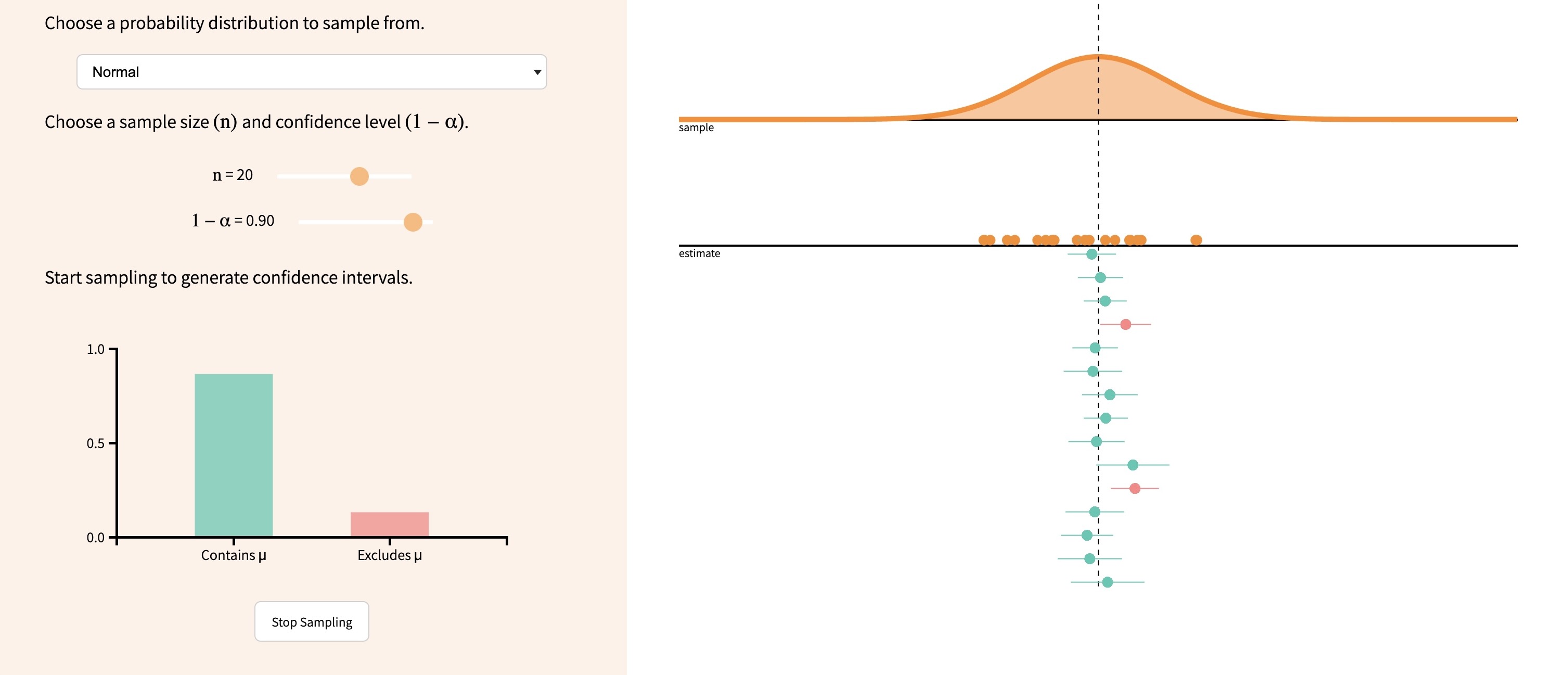
How Many is “Many”?
Code
library(ggplot2)
library(tibble)
library(dplyr)
set.seed(5100)
n_vals <- c(ceiling(sqrt(10)), 10, ceiling(10*sqrt(10)), 100, ceiling(100*sqrt(10)), 1000, ceiling(1000*sqrt(10)), 10000, ceiling(10000*sqrt(10)), 100000)
heads_data <- c()
total_data <- c()
for (n in n_vals) {
  coin_flips <- rbinom(n, 1, 0.5)
  num_heads <- sum(coin_flips)
  heads_data <- c(heads_data, num_heads)
  num_flipped <- length(coin_flips)
  total_data <- c(total_data, num_flipped)
}
results <- tibble(n = n_vals, heads=heads_data, total=total_data)
results <- results %>% mutate(head_prop = heads / total)
#results
ggplot(results, aes(x=n, y=head_prop)) +
  geom_hline(aes(yintercept=0.5, linetype='dashed'), color=cbPalette[2]) +
  geom_line(aes(color='black'), fill=cbPalette[1], linewidth=g_linewidth, color=cbPalette[1]) +
  geom_point(aes(color='black'), size=g_pointsize*0.9) +
  scale_color_manual("", values=c("black","purple"), labels=c("Mean of n samples","Expected Value")) +
  scale_linetype_manual("", values="dashed", labels="Expected Value") +
  scale_fill_manual("", values=cbPalette[1], labels="95% CI") +
  dsan_theme("full") +
  theme(
      legend.title = element_blank(),
      legend.spacing.y = unit(0, "mm")
  ) +
      labs(
          title = "Estimates of Population Mean for Increasing Sample Sizes",
          x = "n (Sample Size)",
          y = "Sample Mean"
      ) +
  scale_x_log10(breaks = c(10, 100, 1000, 10000, 100000), labels = c("10", "100", "1000", "10000", "100000"))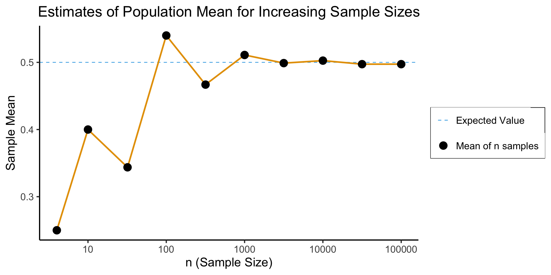
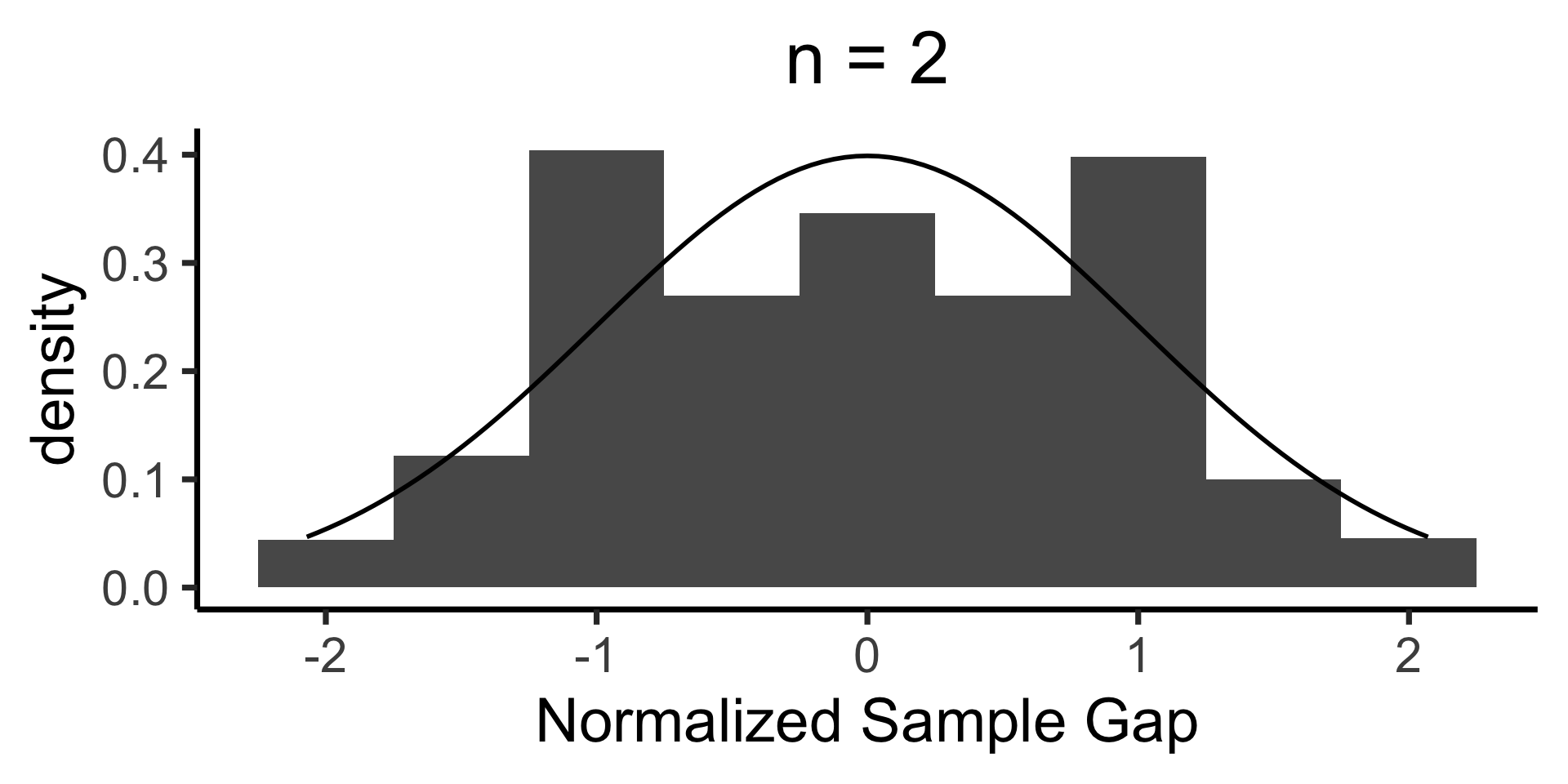
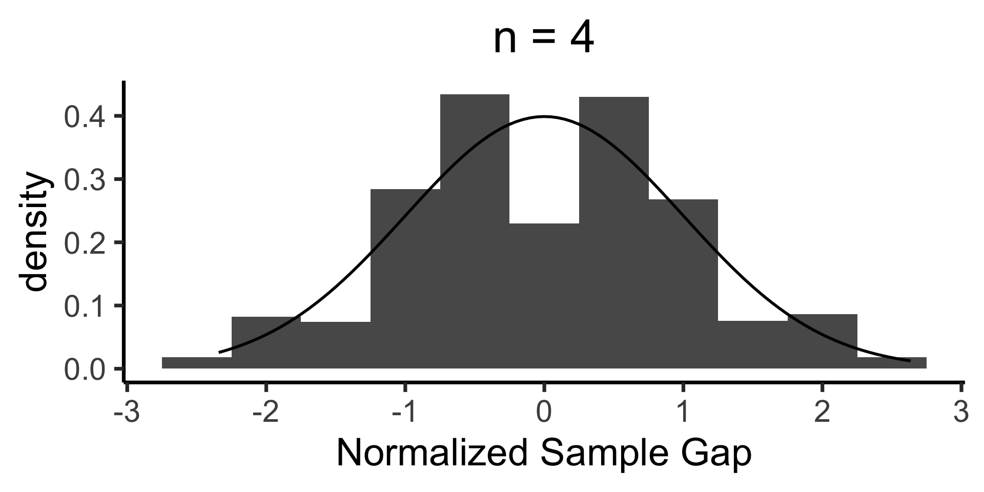
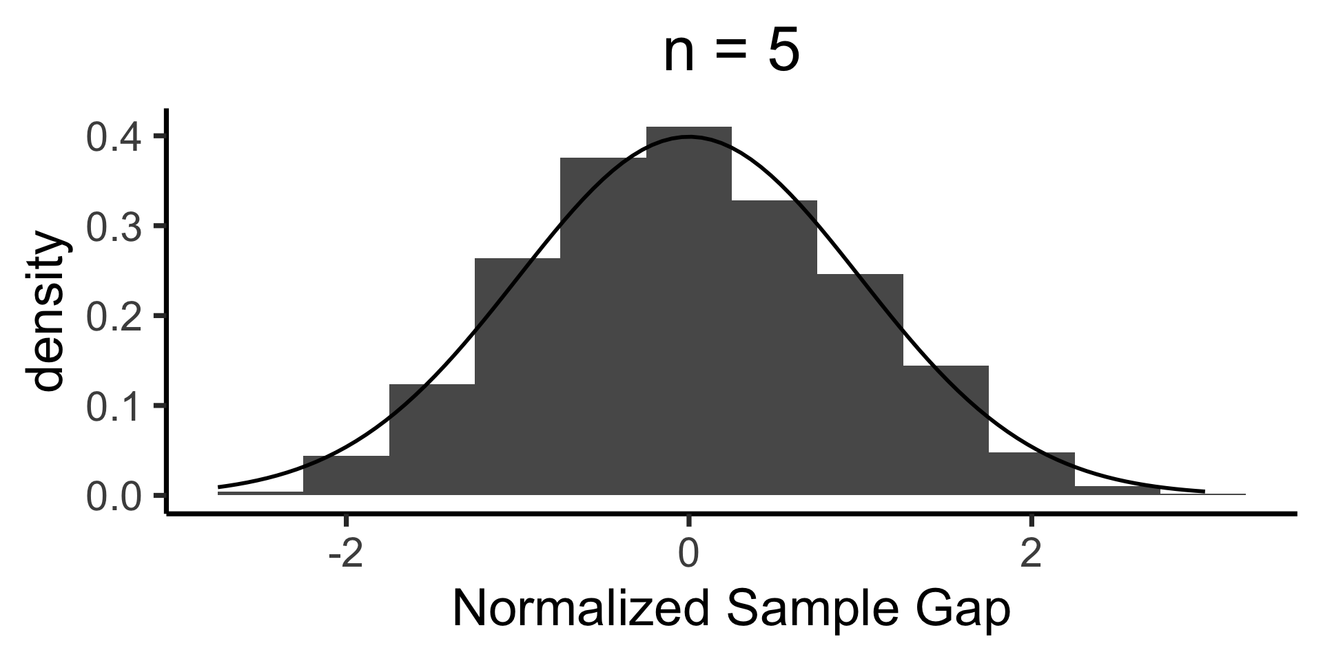
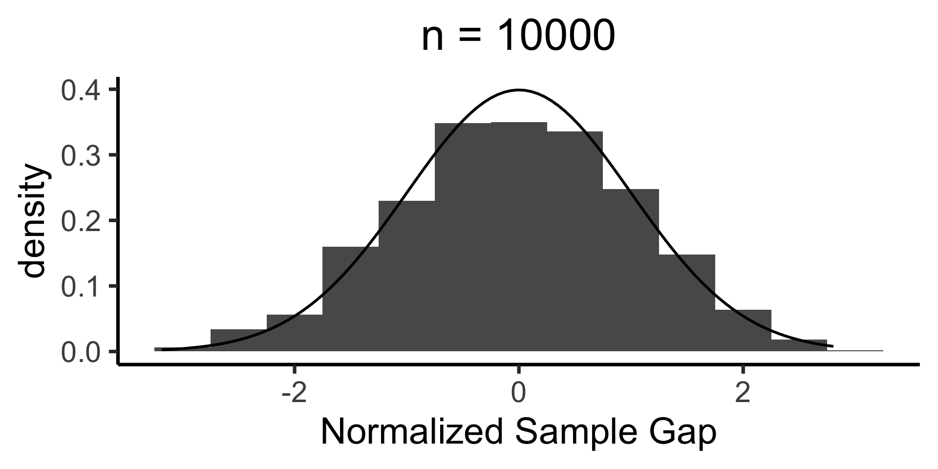
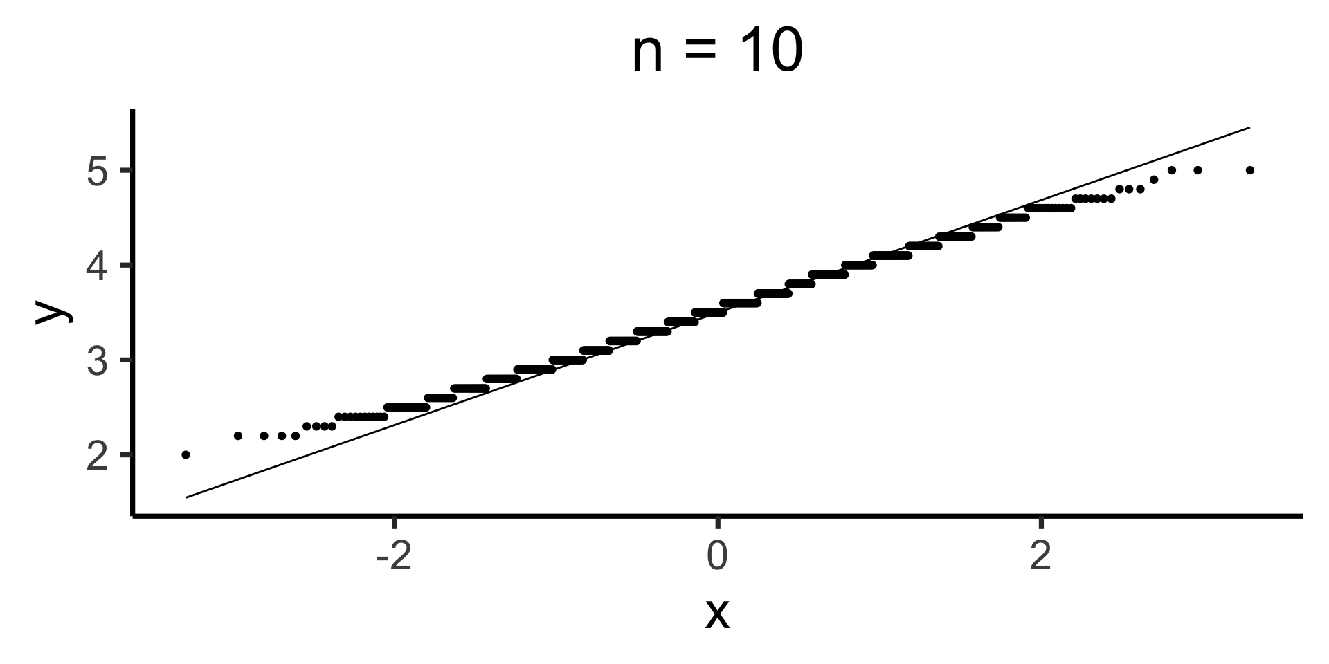
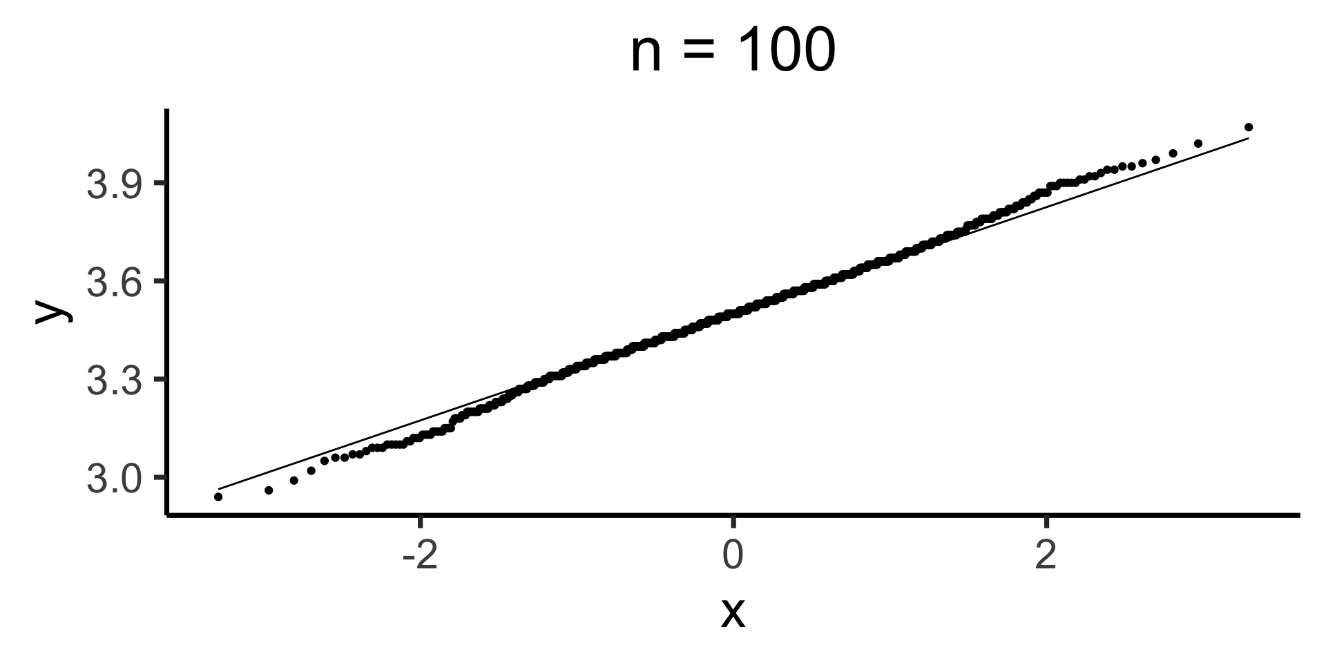
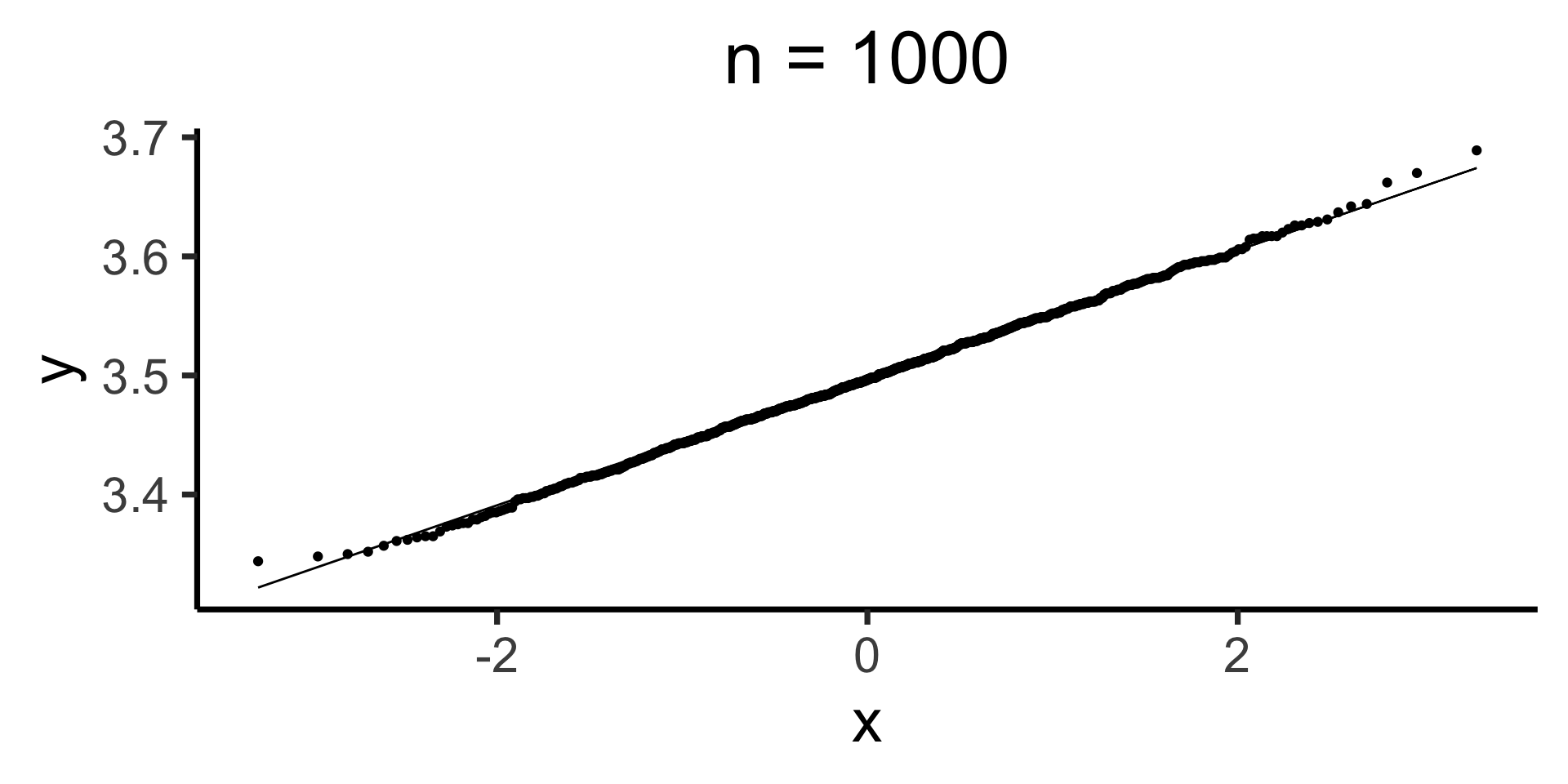
When is \(\mathcal{N}(0, 1)\) a “good” approximation?
Code
# Prepare data for all plots
max_n <- 10000
num_reps <- 1000
all_rolls <- replicate(
  num_reps,
  sample(1:6, size = max_n, replace = TRUE, prob = rep(1 / 6, 6))
)
gen_clt_plot <- function(n) {
  exp_val <- 3.5
  sigma <- sqrt(35/12)
  denom <- sigma / sqrt(n)
  # Get the slice of all_rolls for this n
  n_rolls <- all_rolls[1:n,]
  sample_means <- colMeans(n_rolls)
  norm_gaps <- (sample_means - exp_val) / denom
  n_df <- tibble(norm_gap=norm_gaps)
  #if (n == 5) {
  #  print(sample_means)
  #  print(n_df)
  #}
  ggplot(n_df, aes(x = norm_gap)) +
  geom_histogram(aes(y = after_stat(density)), binwidth = 1/2) +
  #geom_density() +
  stat_function(fun=dnorm, size=g_linesize) +
  dsan_theme("quarter") +
  labs(
    title = paste0("n = ",n),
    x = "Normalized Sample Gap"
  )
}
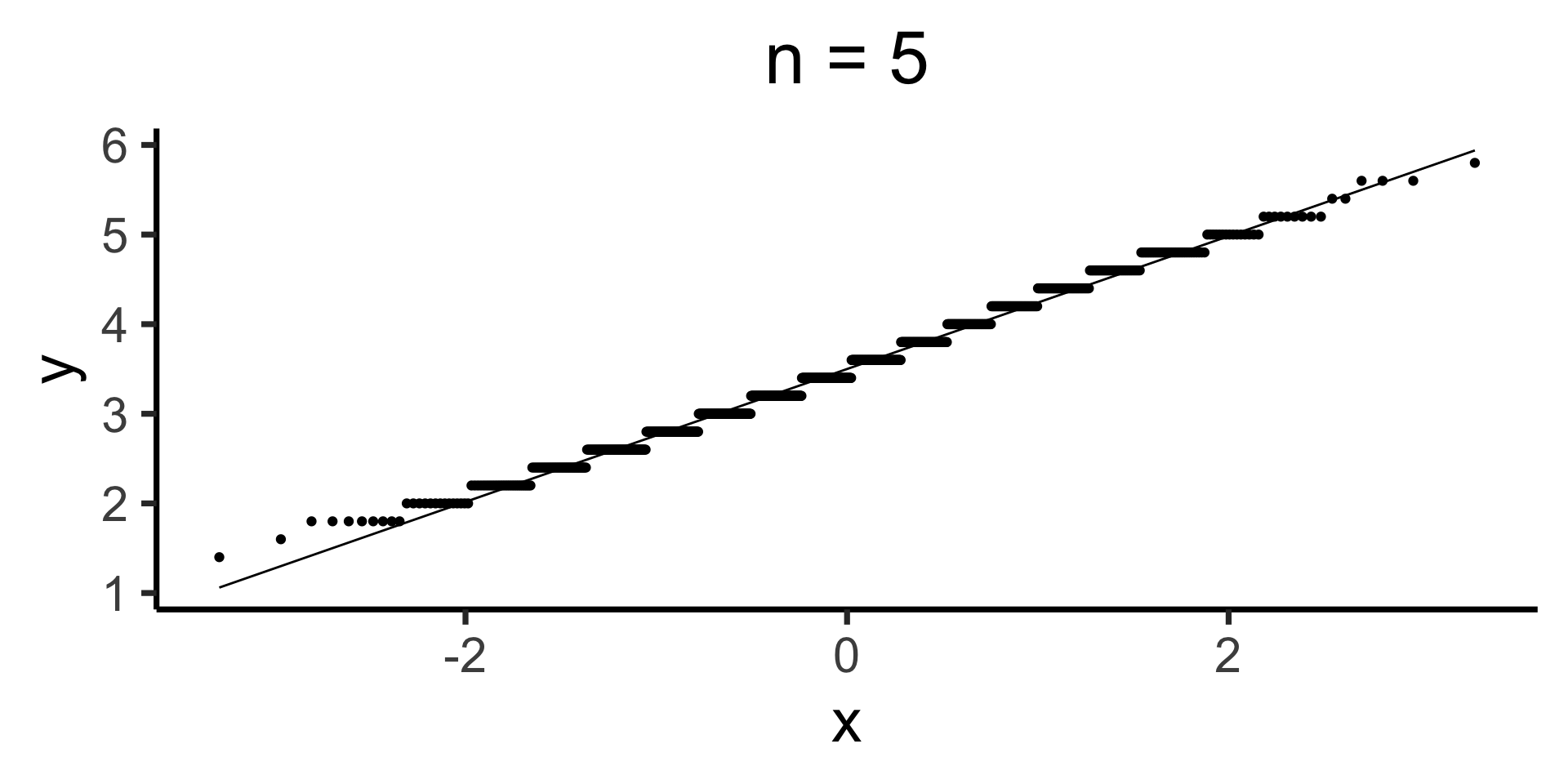
Q-Q Plots
Generative Models
Given a choice of \(\param{\theta}\), we can generate simulated datasets (here 10 for each labeled value of \(\param{p}\)), then compute likelihood as proportion of datasets with 8 heads, 2 tails
From plot: (Among these vals) \(\param{p} = 0.8\) is maximum likelihood estimate

Math Magic 2
2. How do we maximize the product?
\[ p^* = \argmax_{\param{p}} f(\param{p}) \implies f'(p^*) = 0 \]
To maximize likelihood, we need to find its derivative1, set equal to 0, and solve:
\[ \begin{align*} &\frac{d}{d\param{p}}\lik(x \mid \param{p}) = 0 \iff \\ &\frac{d}{d\param{p}}\left[\lik(x_1 \mid \param{p})\lik(x_2 \mid \param{p})\cdots \lik(x_n \mid \param{p})\right] = 0 \end{align*} \]
21st-Century Solution
- Be Bayesian, use priors on parameters (creating hyperparameters)!
- Pretend we know \(\sigma^2\), but want to find the “best” value of \(\mu\):
\[ \begin{array}{rlccc} X_1, X_2 \overset{iid}{\sim} \mathcal{N}( &\hspace{-5mm}\mu\hspace{0.5mm}, &\hspace{-8mm}\overbrace{\sigma^2}^{\large\text{known}}\hspace{-2mm}) & & \\ &\hspace{-4mm}\downarrow & ~ &\hspace{-10mm}{\small\text{estimate}} & \hspace{-6mm} & \hspace{-8mm}{\small\text{uncertainty}} \\[-5mm] &\hspace{-5mm}\mu &\hspace{-5mm}\sim \mathcal{N}&\hspace{-7mm}(\overbrace{m}&\hspace{-12mm}, &\hspace{-16mm}\overbrace{s}) \end{array} \]

The Bias-Variance Tradeoff
But modern Machine Learning basically gets us rly close to a free lunch
 Jeff
Jeff
Intuition
| Low Variance | High Variance | |
|---|---|---|
| Low Bias |  |
 |
| High Bias |  |
 |
In Practice
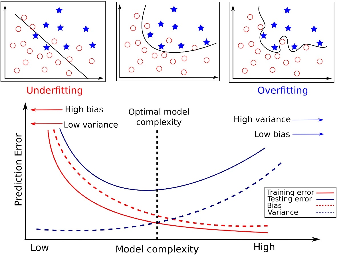
Figure from Tharwat (2019)