Code
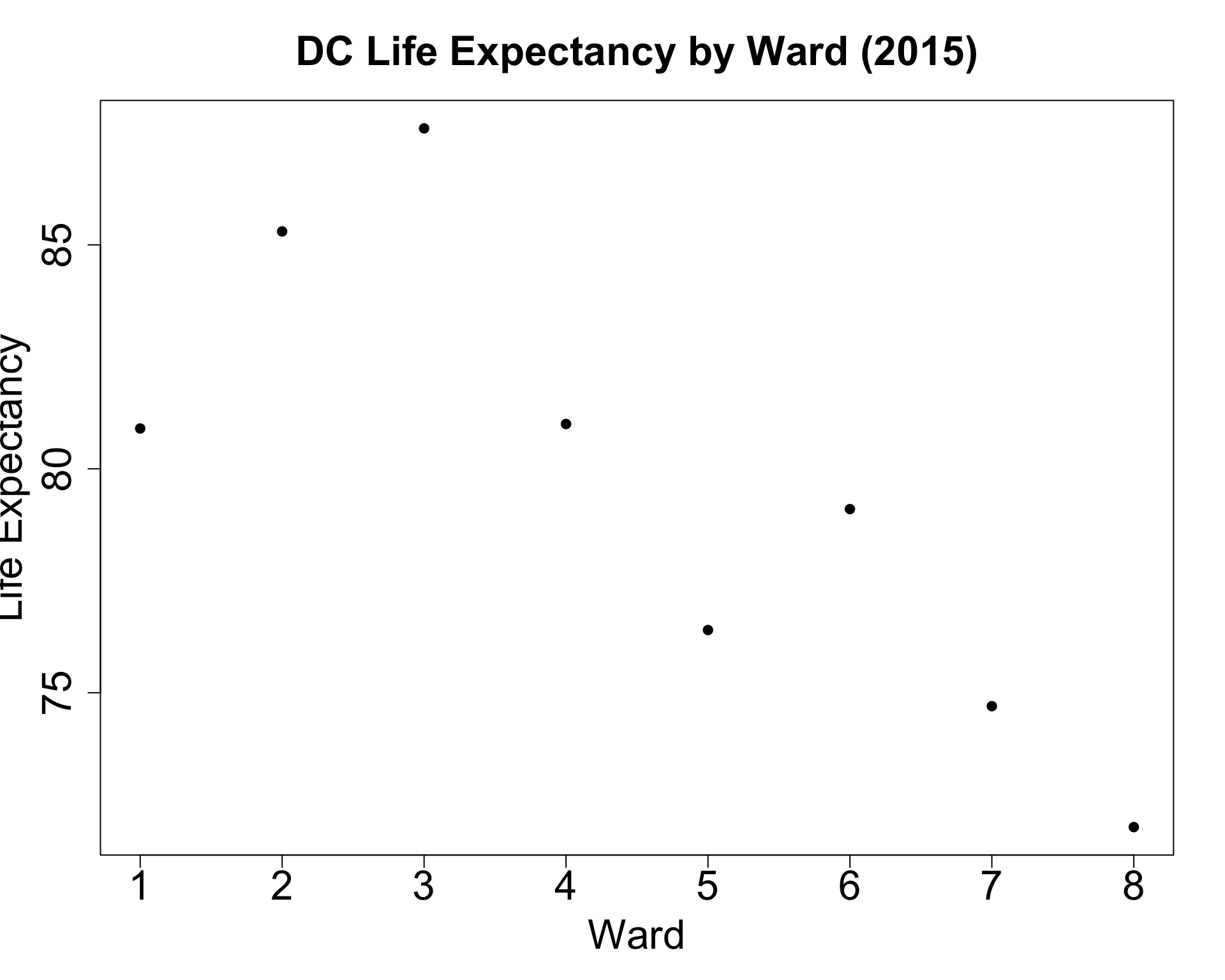
Week 8, Part 1
library(tidyverse)
us_mean <- 78.69
lexp_df <- read_csv("assets/lexp_by_ward.csv")
lexp_df <- lexp_df |> mutate(
  above_avg = ifelse(life_exp > us_mean, "Above Mean", "Below Mean")
)
lexp_df |> ggplot(aes(x=as.factor(ward), y=life_exp, color=above_avg)) +
  geom_point(size=5) +
  geom_segment(
    aes(xend=ward, yend=us_mean),
    linewidth=1.5
  ) +
  geom_hline(
    aes(
      yintercept=us_mean,
      linetype="National Mean"
    ),
    linewidth=1
  ) +
  dsan_theme("half") +
  theme(
    plot.title = element_text(hjust = 0.5)
  ) +
  labs(
    x = "Ward",
    y = "Life Expectancy",
    title = "DC Life Expectancy by Ward (2015)"
  ) +
  scale_linetype_manual("test", values=c("dashed")) +
  remove_legend_title()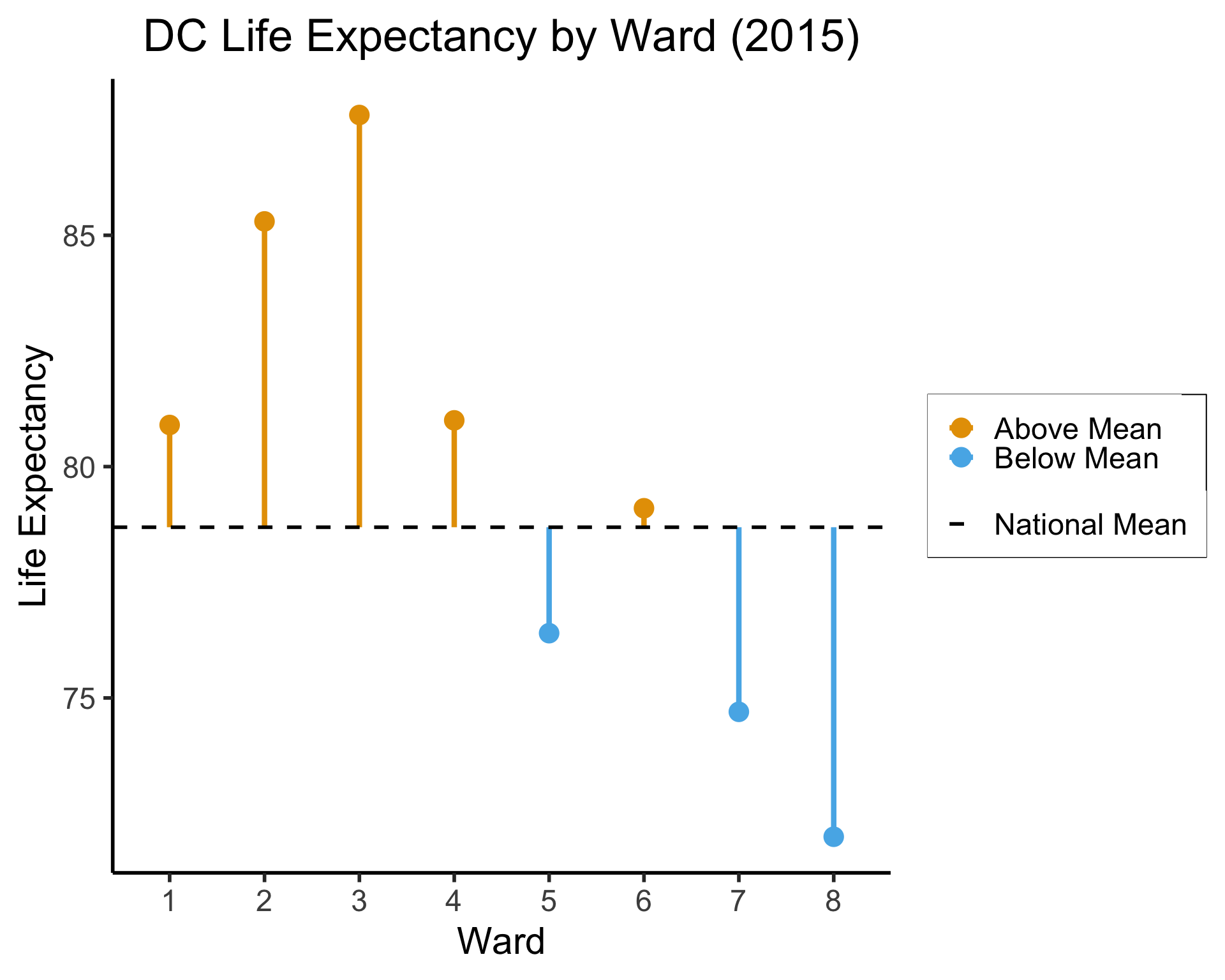
(All using the same syntax)
library(sf)
my_sf <- read_sf("assets/Wards_from_2022.geojson")
my_sf_merged <- my_sf |> left_join(
  lexp_df, by=c("WARD"="ward")
)
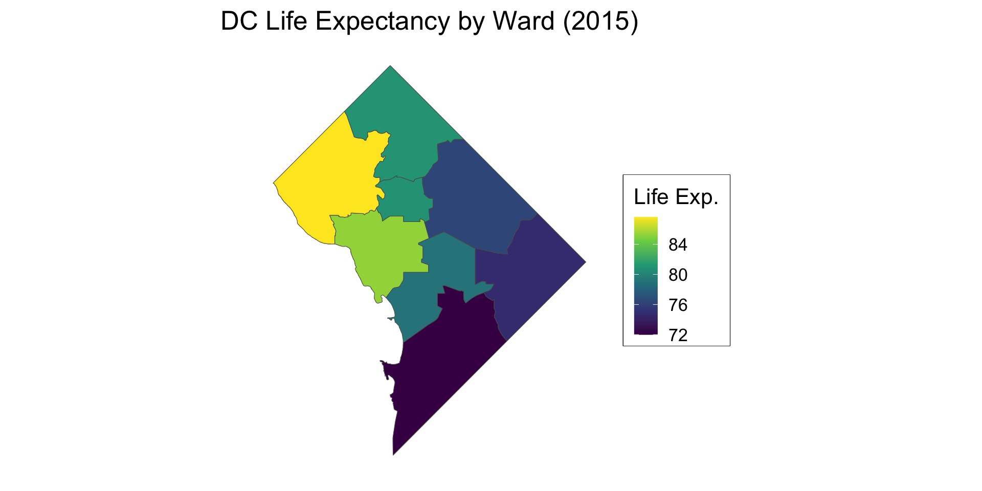
my_sf_merged |> ggplot(aes(fill=life_exp)) +
  geom_sf() +
  dsan_theme() +
  theme(
    axis.line = element_blank(),
    axis.text = element_blank(),
    axis.ticks = element_blank()
  ) +
  labs(
    title = "DC Life Expectancy by Ward (2015)",
    fill = "Life Exp."
  ) +
  scale_fill_viridis_c()
Figure 1: Life expectancy by ward; Shapefile from OpenData.DC.gov
library(tidyverse)
library(datasets)
anscombe_df <- datasets::anscombe |>
  #mutate(id = row_number()) |>
  pivot_longer(
    everything(),
    cols_vary = "slowest",
    names_to = c(".value", "Dataset"),
    names_pattern = "(.)(.)"
  )
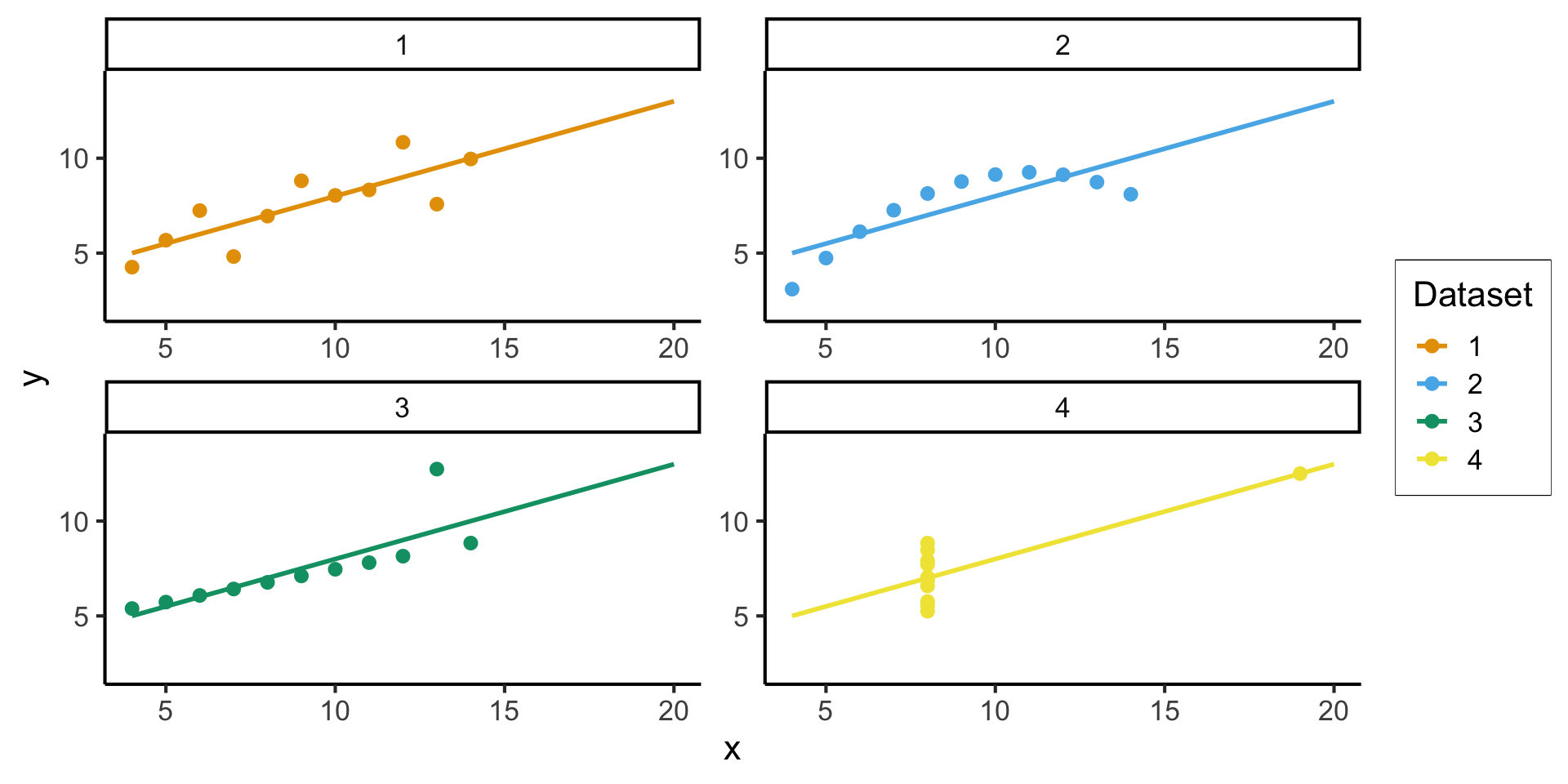
anscombe_plot_base <- anscombe_df |>
  ggplot(aes(x=x, y=y, color=Dataset)) +
  geom_point(size=g_pointsize / 2) +
  geom_smooth(method="lm", se=FALSE, fullrange=TRUE) +
  dsan_theme("full") +
  xlim(c(4, 20)) + ylim(c(2, 14))
anscombe_plot_base +
facet_wrap(vars(Dataset), nrow=2, scales="free")ggplot2 In Practice(In practice, a few central graphical primitives you’ll use over and over again)
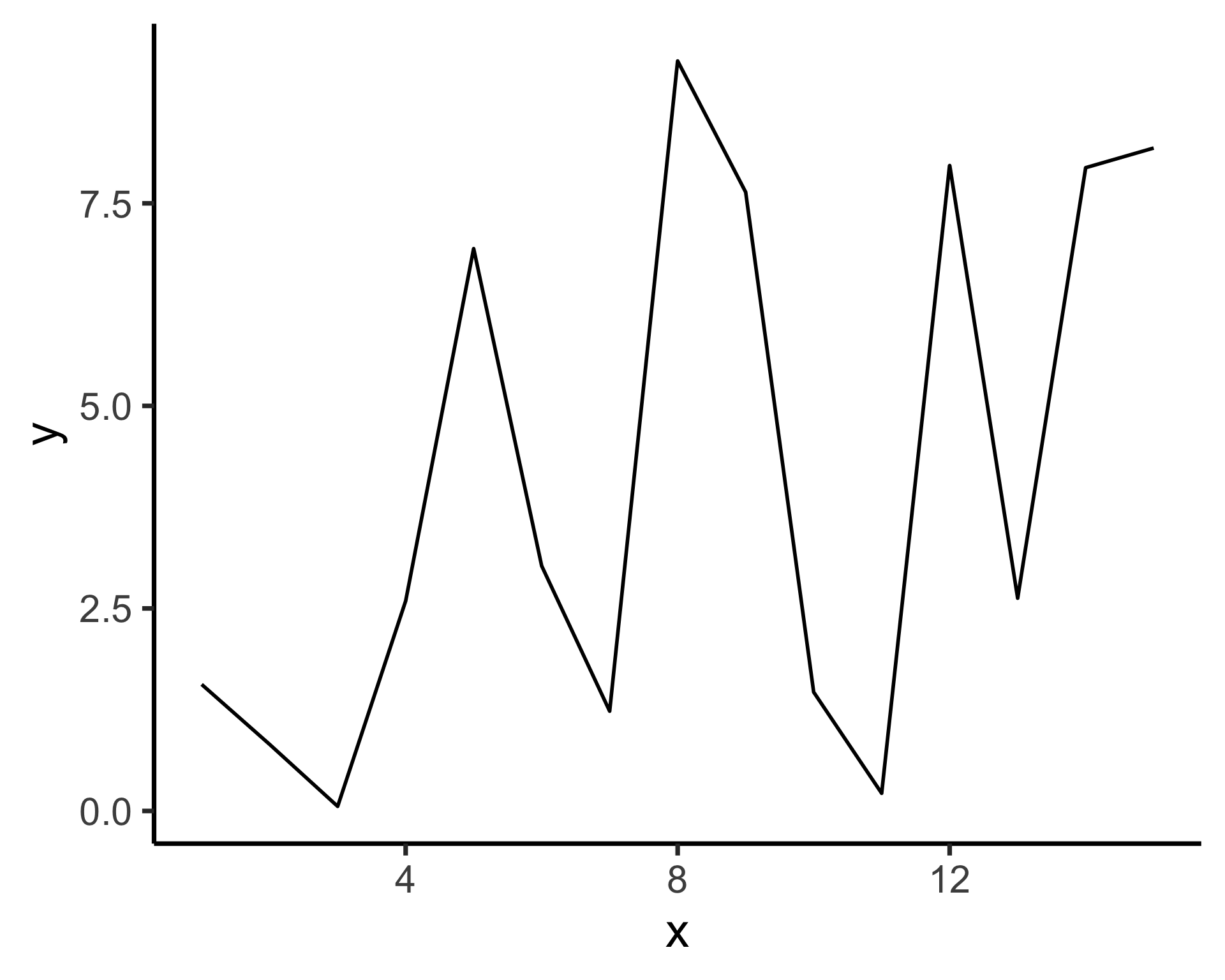
geom_point() for scatterplots
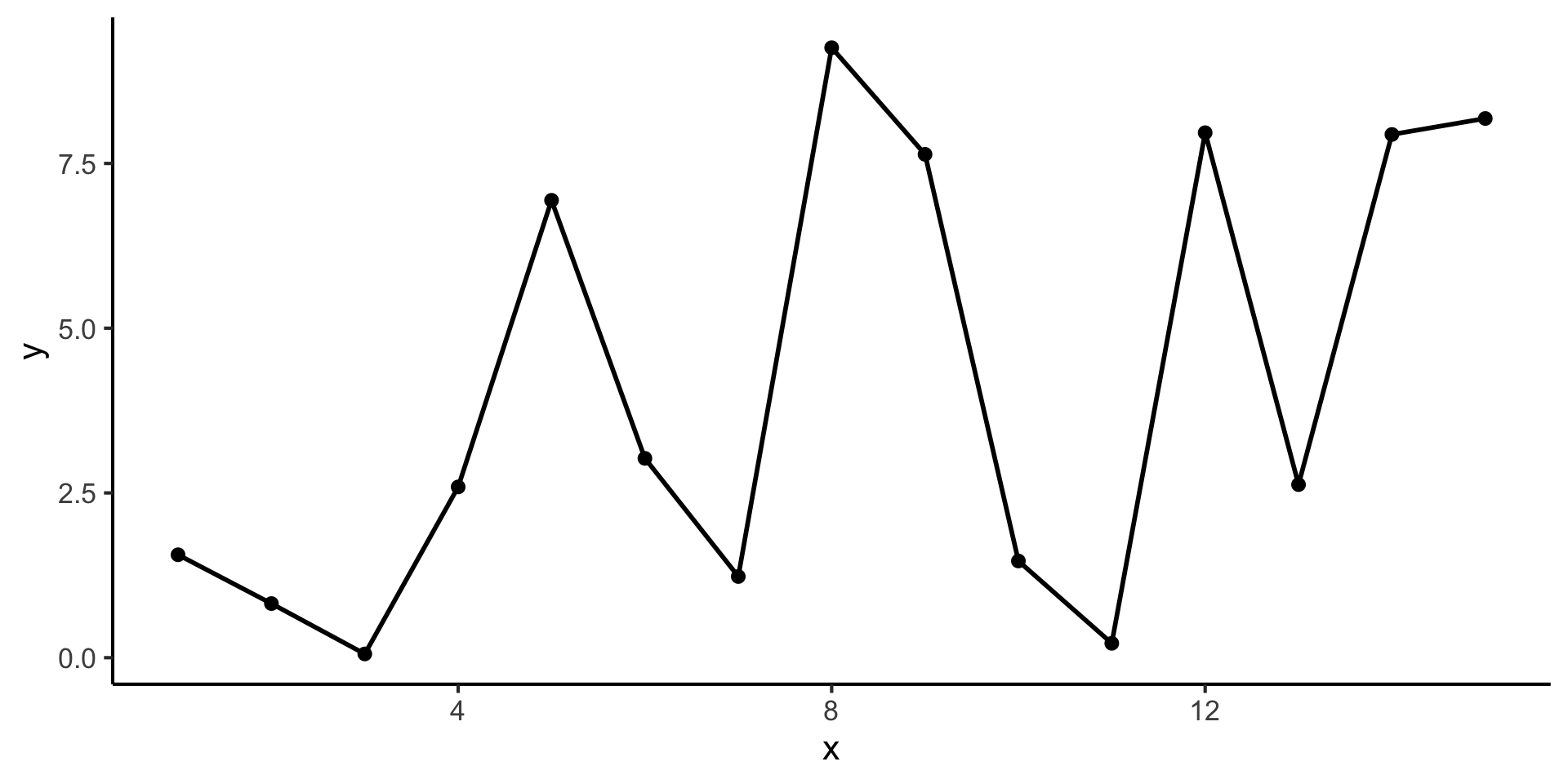
…Which can be used together in a single plot:
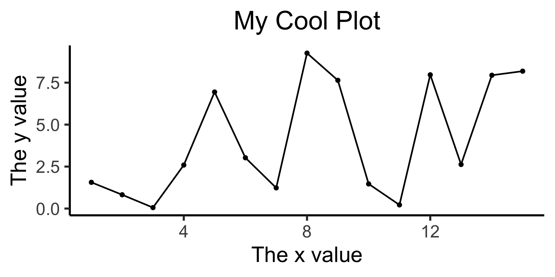
Can all be accomplished using the labs() function!
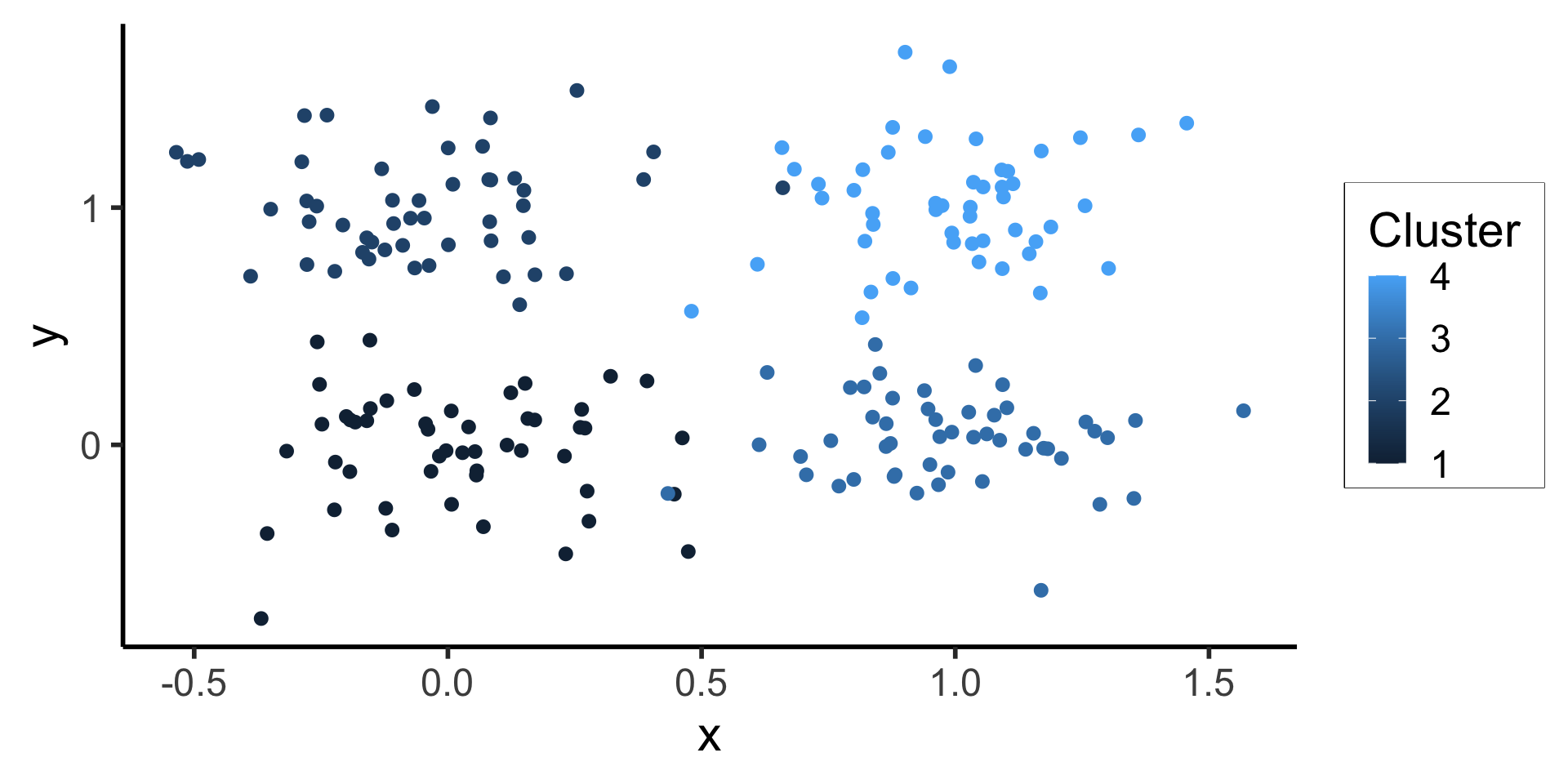
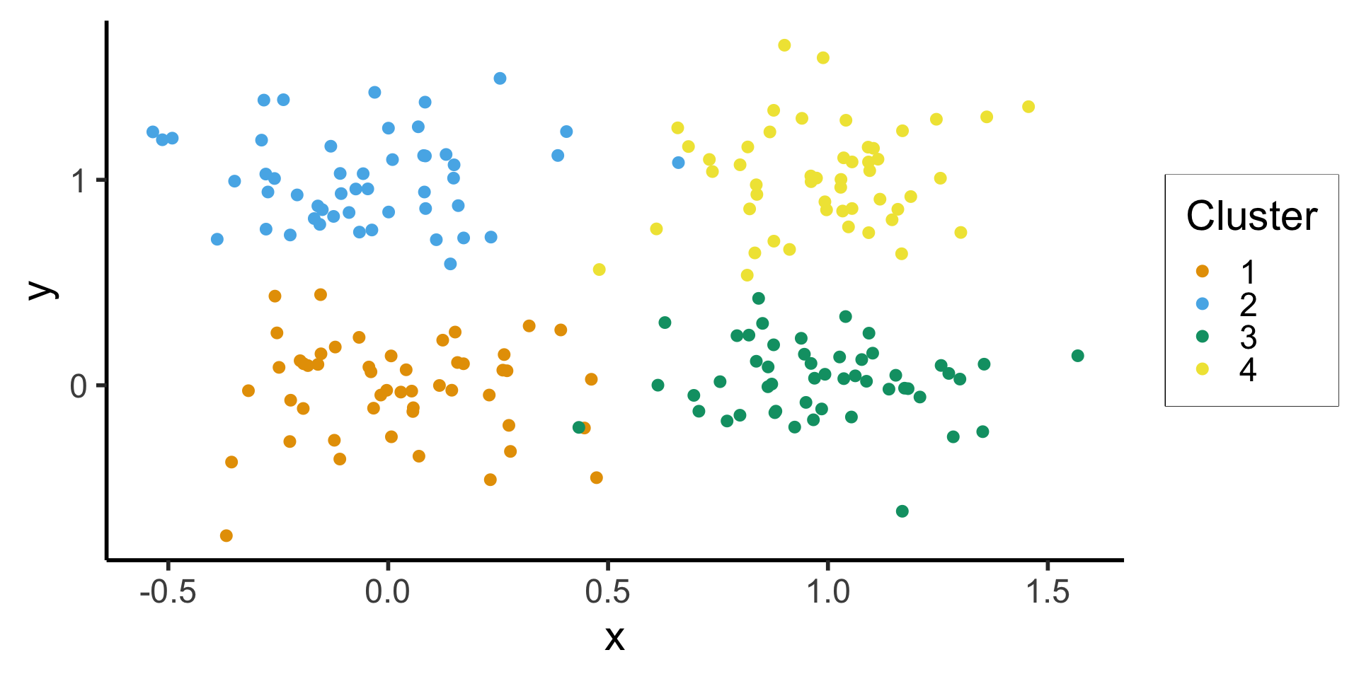
Use the color aesthetic with factor() to differentiate categories
set.seed(2024)
centroids <- list(c(0,0),c(0,1),c(1,0),c(1,1))
cluster_df <- tibble()
N <- 50
Sigma <- matrix(c(0.05, 0, 0, 0.05), nrow=2, ncol=2, byrow=TRUE)
for (i in 1:length(centroids)) {
  cur_centroid <- centroids[[i]]
  # Generate N points from this centroid
  cur_data <- MASS::mvrnorm(N, cur_centroid, Sigma)
  colnames(cur_data) <- c("x", "y")
  cur_df <- as_tibble(cur_data)
  cur_df <- cur_df |> mutate(
    cluster = i
  )
  cluster_df <- rbind(cluster_df, cur_df)
}
Without factor() 
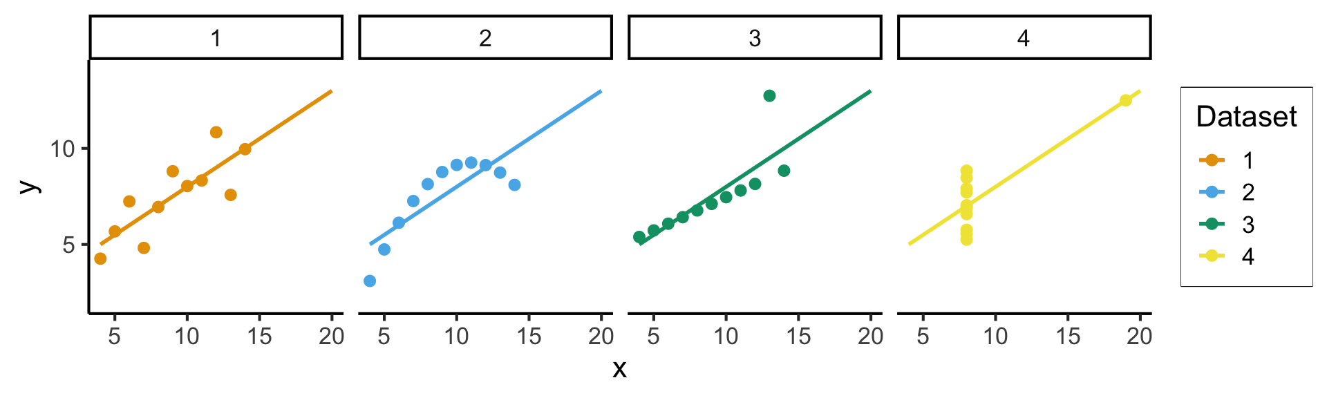
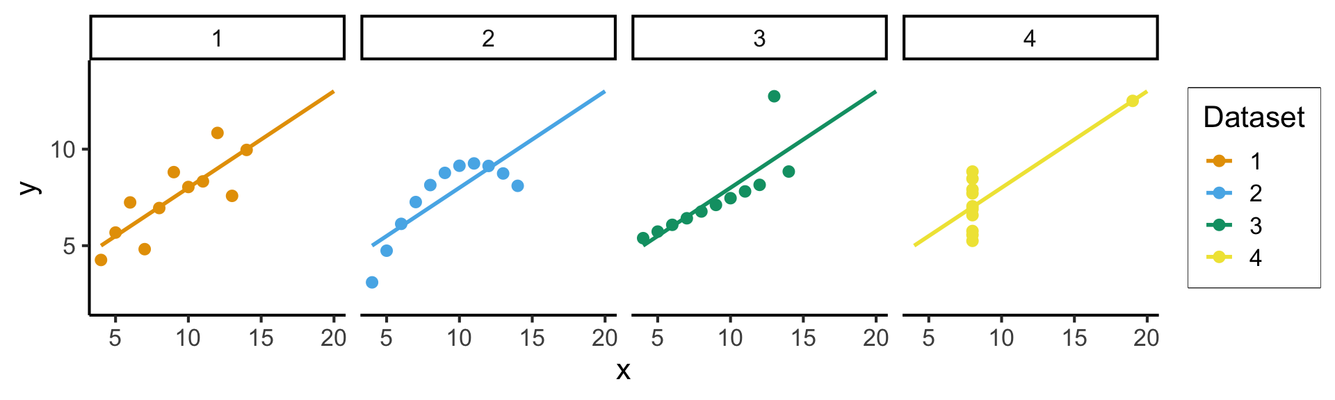
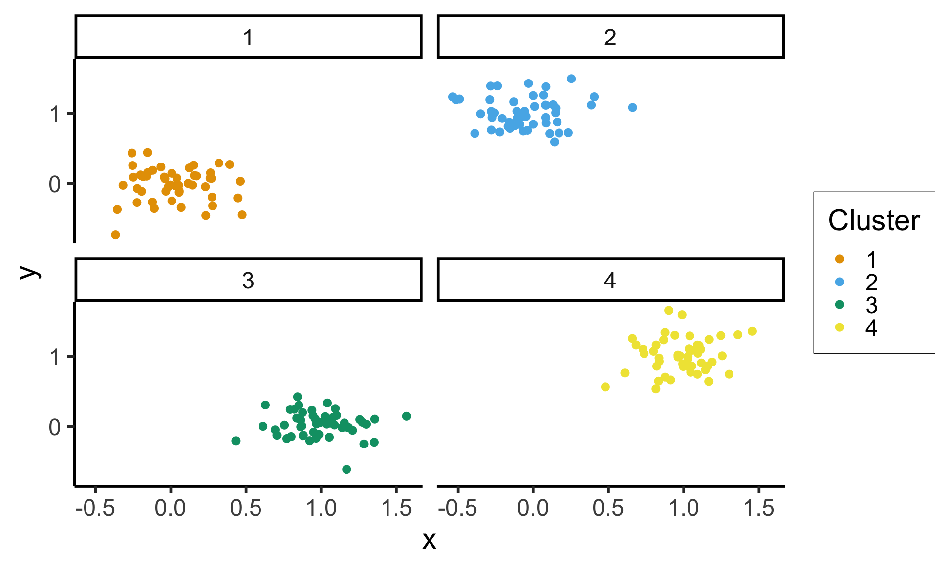
If individual plot gets too busy, facets provide an easy way to split data into multiple (automatically-labeled) plots!
(Much more on this in DSAN 5200: Advanced Data Visualization 😉)