Hello
Please run this code 5 times
Hello
Please run this code 5 times
Hello
Please run this code 5 times
Hello
Please run this code 5 times
Hello
Please run this code 5 timesControl Flow in R
Week 7, Part 1
Jeff Jacobs
DSAN Summer Bootcamp 2024
Georgetown University
Control Flow
In case you haven’t heard this term…
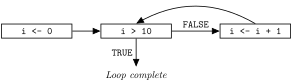
Control flow is just the idea of: how do we control the flow of program execution (individual statements or blocks) in [programming language]
![]()
![]()
Code Blocks
Python uses Indentation →→
R uses curly braces {}
[1] "Hello"
[1] "Please run this code 5 times"
[1] "Hello"
[1] "Please run this code 5 times"
[1] "Hello"
[1] "Please run this code 5 times"
[1] "Hello"
[1] "Please run this code 5 times"
[1] "Hello"
[1] "Please run this code 5 times"
Conditional Statements
If Statements
library(lubridate)
cur_time <- Sys.time()
writeLines(paste0(
    "The current time is ",
    hour(cur_time),":",
    minute(cur_time)
))
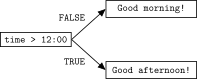
The current time is 17:32if (hour(cur_time) < 12) {
print("Good morning!")
} else if (hour(cur_time) < 18) {
print("Good afternoon!")
} else {
print("Good evening!")
}[1] "Good afternoon!"(We’ll learn about lubridate soon!)
The Ternary Operator
Loops
For Loops: The Software Engineer’s Bread and Butter
- Many different ways to loop (find one that clicks for you!)
- For loops often the “default” approach (because of
C)
Vectorized Operations: The Data Scientist’s Bread and Margarine
- You’ve been hired as the lead data scientist for a food delivery service (congrats!)
- You’re given data on (a) miles traveled and (b) hours driven, for each driver
- Your goal: find the distribution of average speeds!
The Loop Approach ![]()

for (i in 1:nrow(driver_df)) {
  driver_df[i, 'mph'] <- driver_df[i, 'miles'] / driver_df[i, 'hrs']
}
driver_df| miles | hrs | mph |
|---|---|---|
| 11 | 2 | 5.50000 |
| 52 | 3 | 17.33333 |
| 13 | 5 | 2.60000 |
- It works! But CPUs have hyper-optimized linear algebra
- \(\implies\) Operations on a length-1000 vector significantly faster than a loop performing an operation 1000 times
The Vectorized Approach 💯
Vectorizing Your Brain
- Thinking in terms of vectors will be annoying at first! Many common algorithms are “naturally” described via loops…
- It will pay off over the course of your career, I promise!
- (For \(N = 100K\), 0.006 vs. 9.08 seconds!)
How is it That Much Faster?
- The long answer: take DSAN 5500 😜 The short answer:
- Simple math operations (addition, multiplication) are easily parallelized under the hood;
- Sequential memory reads are significantly faster than non-sequential reads—vectors can be stored in contiguous “chunks” of memory that computer can rapidly scan over
- (Think of how it’s easier to count people standing in a line than people scattered around a room!)
Functions
Anonymous Functions
- In Python you declare the name of a function using
def - In R, you make the function without a name, then assign it to a variable:
- (Python also has anonymous functions, via
lambda:)
Variable Scope
- Huge point (especially for Week 7 Assignment)!
- Think of functions as “mini-programs”, where variables (including arguments) get created when the function starts and then destroyed when the function finishes. Compare:
Positional vs. Keyword Arguments
- Just like Python, R functions can accept two types of arguments…
Positional arguments are required (function call will produce error if any positional argument is missing)
Applying Functions to Vectors
- We’ve been “manually” calling functions, like
func(arg) - What if we want to apply a function to a vector of elements? Ex: capitalize a big list of names
- Base R provides a family of
apply()functions:sapply()for vectors;lapply()for lists;apply()for matrices (requires specifying axis: columns or rows)
2024 DSAN Bootcamp W07-1: Control Flow